|
|||||
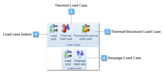
Load case button
Create a load case
A load case is then created including the selected loads (multiplied by coefficients if needed) plus boundary conditions and solution controls (for nonlinear analysis). In this way, the complete loading history can be defined.
Load cases must be generated when all load groups are defined prior to the solving process in order to obtain results. Load group definition is not enough by itself obtain results and an error message will appear if at least one load case is not created.
Each load case is independent from each other. All loads about to be solved must be included in the corresponding load case. If a load is not included in a load case it won't be taken into consideration in the solution process.
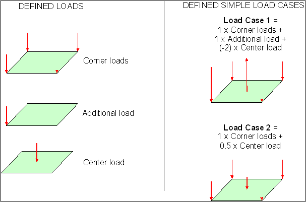
An example of a CiviFEM load case would be the following:
LoadCase1 = 1 x Corner Loads + 1 x Additional Loads – 2 x Center Load
LoadCase2 = 1 x Corner Loads + 0.5 x Center Load
A load case is composed of:
The structural load case table description shows different options that are not available neither in a thermal nor in a seepage load case:
When Turn off dynamic effects is activated in a structural transient analysis the load case is solved at as a static structural one. This is very useful in case you have initial loads like gravity. In this case define the first load case with the loads that you don´t desire to have dynamic effects and activate the checkbox in the load case option.
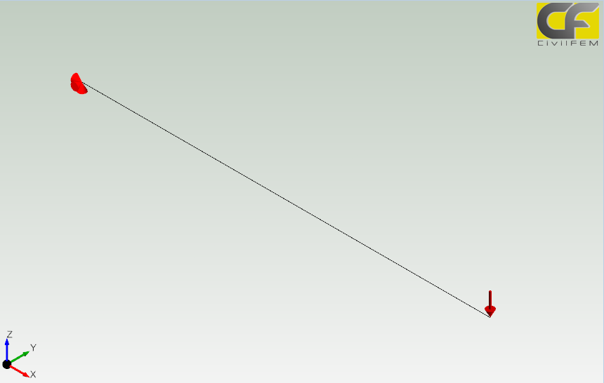
When the option Generate a TXT results file is active, during the solving process a .txt results file with the result information is carried out. The next model consists of a beam structural element embedded on one end while a load is applied on the cantilever.
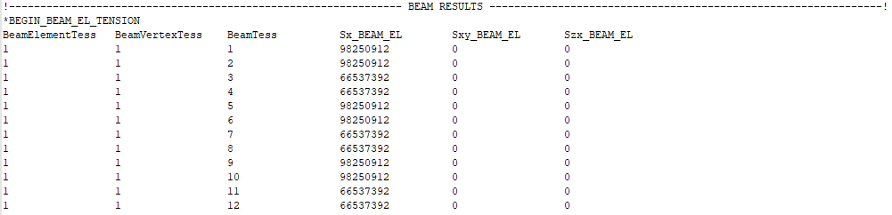
Once this model has been solved, a new .txt file has been performed. This file will contain the result information of this model. For instance, this .txt model should have written the stresses all along the beam structural element. Therefore if the .txt file is checked, this would be a little piece of information contained on it:
The target of getting this information is to attach the .txt file to a new calculation process so as that taking into account the previous solving process results. For this purpose it is necessary to load this file on the initial state tool, on the solve ribbon. The process has been detailed on this solve toolbar chapter: Initial State Toolbar. This property will be only available if the model is a structural one.
Another way to reproduce the initial state of a model is to Reset the displacements to zero generated by the gravity for example. A typical example of this method can be how to generate the stress field in a soil, where the gravity is applied but no displacements occurs in this initial state. To model this example, user must create a first load case with the gravity applied, then in the second load case (with gravity also applied) reset displacement option must be activated.
When reset displacement to zero is activated use can select for previous load cases Use elastic Geomaterials or not to solve them.
The procedure to reset the displacement in CivilFEM is by creating internal load cases that are solved in order to reset the displacement but maintaining the stresses. First a load case where all the elements are deactivated and displacements are set to zero, then elements are reactivated and loaded. In case of use elastic geomaterials, the procedure is repeated twice.
On the other hand, the Perform a SSRM analysis option will be only available on a static structural analysis. The user has to take into consideration some aspects before using this utility:
In regard to the last assessment, in first step, the user should carry out the fully structural process, taking as many loading states as necessary to perform the particular situation. The second step would consist of keeping the load state condition of the last load case, besides introducing the SSRM analysis.
The target would be to come out a safety factor. Cohesion and phi parameters, from the Mohr-Coulomb material model, will be divided by this safety factor so, the user will manage to obtain those cohesion and phi values in which the soil reaches to its failure.
In addition, the safety factor grows proportionally with the initial SSRM step fraction so, when solving the load case with the SSRM analysis active, CivilFEM will multiply the calculation time by the pertinent SSRM step fraction. This value will be added to the initial safety factor, which value has been specified as 1.
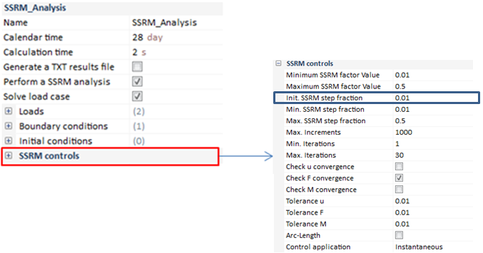
As it can be checked, the Initial SSRM step fraction has been specified as 0.01 so, this value will be multiplied by the calculation time throughout the resolution. For instance, a little explanation will be provided with the next example:
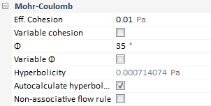
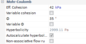
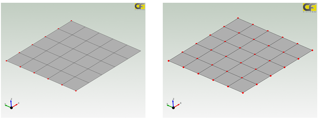
This soil has been modeled with the next scheme of Mohr-Coulomb parameters:
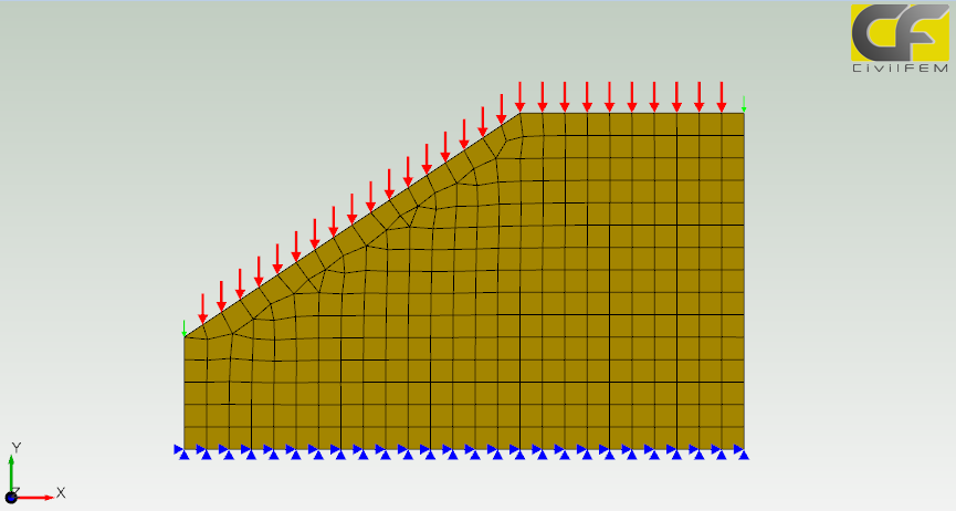
Once the Morh-Coulomb behavior has been established, the user has to define the different load states. For this example, loads into consideration will be a 0.2 Mp/m linear load along with the self weight effect; assigned on the top soil perimeter just as visualized in the previous image. For this purpose, only one load case would become necessary; nevertheless, in order to apply the SSRM analysis, CivilFEM requires the application of a second load case on which both loads and boundary conditions are the same than in the first load case. The difference falls into the activation of the SSRM analysis check box.
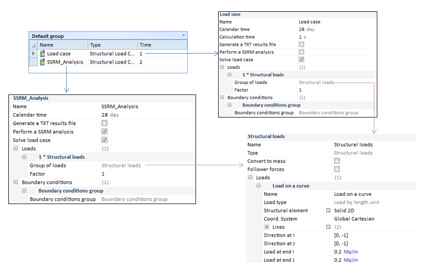
The load state fulfill the assigned load states so that the SSRM analysis can be performed. This last load case will be performed under particular solution controls, activating the instantaneous load control application, as visualized previously. On the other hand, this process will not be applied in case of taking into consideration either variable phi or cohesion.
On other instance, for this example it is necessary to activate the incremental results option because the analysis could not reach to the last increment. Thus, the process stopped calculating in the increment number thirteen. Once the result has been loaded, the data contained in the Information option is available, being the SSRM Factor 1.970. This means that the SSRM step fraction value may be obtained:
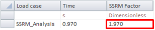
Therefore, cohesion and phi values will be easily obtained:
This means that for lower safety factor values, or higher c and phi values, the convergence would be available.
| ||||||||||||||||||||||||
Thermal Load Case
Create a thermal load case
The concept in a thermal load case is very similar to a structural one. However, in a thermal load case, the capability of adding a load group does not exist due to every thermal load is cataloged as a boundary condition. Therefore, boundary conditions will be the only entity so as to enter in a thermal load case.
At least one Thermal load case has to be created previously to the solving process. Thermal boundary condition definition is not enough by itself to obtain results and an error message will appear if at least one thermal load case is not created. This error message will only appear in case of not having any Thermal Load Case and the analysis class is defined as "thermal" in the Global Solution Controls. On the other hand, if the model ties to be solved defining the analysis class as "structural" and any structural load case has been created, the error message will appear as well.
Each thermal load case is independent from each other. All thermal boundary conditions about to be solved must be included in the corresponding thermal load case. If a thermal BC is not included in a thermal load case it won't be taken into consideration in the solution process.
For instance, the next example will visualized the capability previously described:
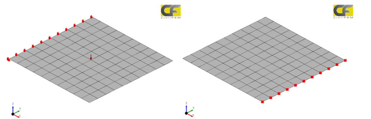
Load case 1:
Load case 2:
Load Case 1 Load Case 2
In the example, two different thermal load cases have been created but in the first one, only a temperature on curves BC has been entered. However, in the second one, it was a temperature on surface. Each thermal load case will be solved separately with the data which correspond, independently.
A thermal load case is composed of:
| ||||||||||||
Thermal/Structural Load Case
Create a thermal/Structural load case
The Thermal/Structural load case allow the user to combine both the structural and the thermal analysis by adding structural load group along with both structural and thermal boundary conditions. This option solves a coupled thermal/structural analysis.
As in the structural analysis, the selected loads may be multiplied by coefficients if needed, besides a thermal initial condition group have to be entered to define the initial environmental condition.
In addition, if the model tries to be solved defining the analysis class as "Thermal/Structural coupled" and any Thermal/Structural load case has been created, the error message will appear as well. This error message will only appear in case of not having any Thermal/Structural Load Case and the analysis class is defined as "Thermal/Structural Load Case" in the Global Solution Controls.
On the other hand, each load case is independent from each other. All loads about to be solved must be included in the corresponding load case. If a load is not included in a load case it won't be taken into consideration in the solution process.
For instance, the next example will visualized the capability previously described:
Figure 1: Structural Loads:
Figure 2: Thermal Loads:
Figure 3: Thermal Structural Load case :
Structural Load Case Thermal Load Case
Thermal/Structural Load Case
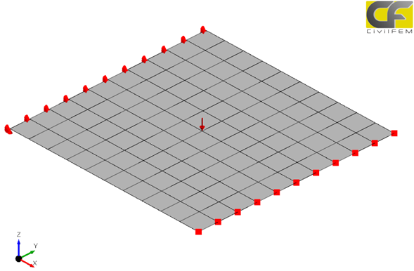
In the example, only a thermal structural load case has been created. This load case contains the structural load and the structural boundary condition along with the thermal boundary conditions. This load case allow the user to solve a thermal structural coupled analysis.
A thermal load case is composed of:
| ||||||||||||||||||
Seepage Load Case
Create a seepage load case
The concept in a seepage load case is very similar to a structural one. However, in a seepage load case, the capability of adding a load group does not exist due to every thermal load is cataloged as a boundary condition. Therefore, boundary conditions will be the only entity so as to enter in a seepage load case.
At least one seepage load case has to be created previously to the solving process. Seepage boundary condition definition is not enough by itself to obtain results and an error message will appear if at least one seepage load case has not been created. This error message will only appear in case of not having any Seepage Load Case and the analysis class is defined as "seepage" in the Global Solution Controls. On the other hand, if the model ties to be solved defining the analysis class as "structural" and any structural load case has been created, the error message will appear as well.
Each seepage load case is independent from each other. All the seepage boundary conditions about to be solved must be included in the corresponding seepage load case. If a seepage BC is not included in a seepage load case it won't be taken into consideration in the solution process.
For instance, the next example will visualized the capability previously described:
Load case 1:
Load case 2:
Load Case 1 Load Case 2
In the example, two different seepage load cases have been created but in the first one, only a total head on curves BC has been entered. However, in the second one, it was a total head on surface. Each seepage load case will be solved separately with the data which correspond, independently.
A seepage load case is composed of:
| ||||||||||||
