Finite element characteristics

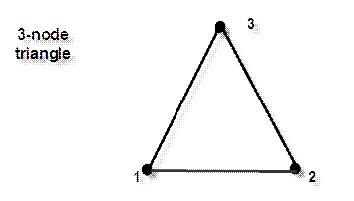
Depending on the structural element selected (and cross section material) different element types are available from CivilFEM library: 2-node linear beam with transverse shear, 8-node quadrilateral, 3-node triangle, 8-node hexahedron, etc.

Each element type has unique characteristics governing its behavior . This includes the number of nodes, the number of direct and shear stress components, the number of integration points used for stiffness calculations, the number of degrees of freedom, and the number of coordinates.

User can choose different element types to represent various parts of the structure in an analysis. If there is an incompatibility between the nodal degrees of freedom of the elements, user has to provide appropriate tying constraints to ensure the compatibility of the displacement field in the structure. CivilFEM assists user by providing many standard tying constraint options, but user is responsible for the consistency of the analysis.

Integration points

The CivilFEM program makes use of both standard and nonstandard numerical integration formulas. The particular standard and nonstandard integration formulas used for each finite element matrix or load vector is given in the following corresponding chapters (refer to Chaters 5.3.2 – 5.3.5 ).

For each section, the program provides the location of the integration points with respect to the principal axes and the integration weight factors of each point. Furthermore, it computes the coordinates of the center of gravity and the principal directions with respect to the input coordinate system. It also computes the area and the principal second moments of area of the cross section.

It is not recommended to use solid sections as an alternative to thin-walled sections as underlying assumptions underlining it are not accurate enough to model such sections.It does not account for any warping of the section and, therefore, overestimate the torsion stiffness as it is predicted by the Saint Venant theory of torsion.

In rectangular, trapezoidal and hexagonal solid sections the first integration point is lower left corner and the last is the upper right corner. They are numbered from left to right and then from bottom to top.

The first integration point in each quadrilateral segment is nearest to its first vertex and the last integration point is nearest to its third vertex. They are numbered from first to second then to third vertex.The segments are numbered consecutively in the order in which they have been entered. Thefirst integration point in a new segment simply continues from the highest number in the previous segment. There is no special order requirements for the quadrilateral segments. They meet the previously outlined geometric requirements.

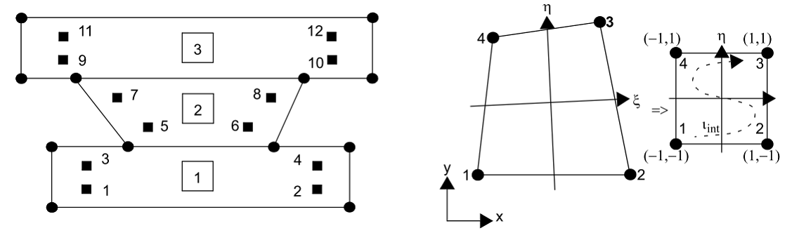
Figure above shows a general solid section constituting of three quadrilateral segments using a 2 x 2 Gauss integration scheme. It also shows the numbering conventions adopted in a quadrilateral segment and its mapping onto the parametric space. For each segment in the example, the first corner point is the lower-left corner and the corner points have been entered in a counterclockwise sense. The segment numbers and the resulting numbering of the integration points are shown in the figure. Gauss integration schemes do not provide integration points in the corner points of the section. Other integration schemes like Simpson or Newton-Cotes schemes exist.

In general, a 2 x 2 Gauss or a 3 x 3 Simpson scheme in each segment suffices to guarantee exact section integration of linear elastic behavior.

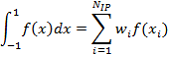
The standard 1-D numerical integration formulas which are used in the element library are of the form:

Where:

f(x)	Function to be integrated
w_i	Weighting factor
x_i	Locations to evaluate function
l	Number of (Gauss) integration points.

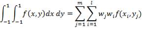
The numerical integration of 2-D quadrilaterals gives:

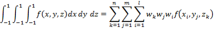
The 3-D integration of bricks and pyramids gives:

1. Truss finite elements

CivilFEM contains 2-node isoparametric truss elements that can be used in three dimensions. These elements have only displacement degrees of freedom.

Since truss elements have no shear resistance, user must ensure that there are no rigid body modes in the system.

Truss type	Reference
3D truss	2 nodes

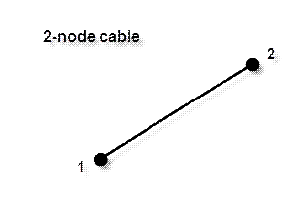
Two-node straight truss

This two-noded element type is a simple straight truss with linear interpolation along the length with constant cross section. The strain-displacement relations are written for large strain, large displacement analysis. All constitutive relations can be used with this element. This element can be used as an actuator in mechanism analyses.

The stiffness matrix of this element is formed using a single point integration. The mass matrix is formed using two-point Gaussian integration.

The interpolation function can be expressed as follows:

Where ψ, ψ are the values of the function at the end nodes and ξ is the normalized coordinate (

. This element has no bending stiffness.

Used by itself or in conjunction with any 3-D element, this element has three coordinates and three degrees of freedom. Otherwise, it has two coordinates and two degrees of freedom.

Connectivity:

Global displacement degrees of freedom:

u	Displacement
v	Displacement
w	Displacement (optional)

2. Beam finite elements

The beam elements are numerically integrated along their axial direction using Gaussian integration. The stress strain law is integrated through thin-walled sections using a Simpson rule and through solid sections using a Simpson, Newton-Cotes, or Gauss rule depending on the input specifications. Stresses and strains are evaluated at each integration point through the thickness. This allows an accurate calculation if nonlinear materialbehavior is present. In elastic beam elements, only the total axial force and moments are computed at the integration points.

The length of a beam element is generally the distance between the last node and the first node of the element.

The orientation of the beam (local x-axis) is generally from the first node to the last node. The local z-axis is normal to the beam axis.

The cross-section axis orientation is important both in defining the beam section and in interpreting the results.

Six degrees of freedom are available for beam finite elements:

U_x	Global Cartesian x-direction displacement
U_y	Global Cartesian x-direction displacement
U_z	Global Cartesian x-direction displacement
θ_x	Rotation about global x-direction
θ_y	Rotation about global y-direction
θ_z	Rotation about global z-direction

When using beam elements, CivilFEM will set the element behavior depending on the beam cross section properties: concrete solid or steel thin section closed and steel open beams.

Beam section type	Reference
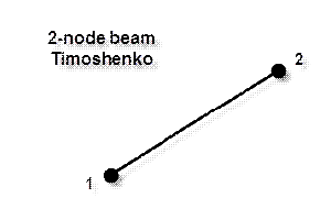
Solid section (concrete)	2 nodes Timoshenko’s theory
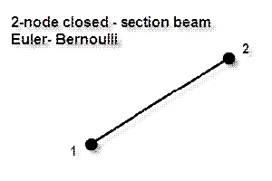
Closed-section (steel)	2 nodes Bernoulli’s theory
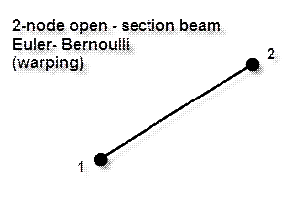
Open-section (steel)	2 nodes Bernoulli’s theory Warping included
2D Case	2 nodes Bernoulli’s theory

Elastic straight Timoshenko solid beam

This is a straight beam in space which includes transverse shear effects with linear elastic material response as its standard material response, but it also allows nonlinear elastic and inelastic material response. Large curvature changes are neglected in the large displacement formulation. Linear interpolation is used for the axial and the transverse displacements as well as for the rotations.

Beam structural elements can be used to model linear or nonlinear elastic response.

Nonlinear elastic response can be modeled when the material behavior is given. Beam elements can also be used to model inelastic and nonlinear elastic material response when employing numerical integration over the cross section. Inelastic material response includes plasticity models, creep models, and shape memory models, but excludes powder models, soil models, concrete cracking models, and rigid plastic flow models. Elastic material response includes isotropic elasticity models and nonlinear elasticity models, but excludes finite strain elasticity models and orthotropic or anisotropic elasticity models.

The element uses a one-point integration scheme. This point is at the midspan location. This leads to an exact calculation for bending and a reduced integration scheme for shear. The mass matrix of this element is formed using three-point Gaussian integration.

Connectivity:

Closed-section Euler-Bernoulli beam

This is a simple, straight beam element with no warping of the section, but includes twist. The default cross section is a thin-walled, closed-section beam.

The generalized strains are stretch, two curvatures, and twist. Stresses are direct (axial) and shear given at each point of the cross section.

Connectivity:

Open-section beam

This is a simple, straight beam element that includes warping and twisting of the section. Primary warping effects are included, but twisting is assumed to be elastic.

The degrees of freedom associated with the nodes are three global displacements and three global rotations, all defined in a right-handed convention and the warping.

The generalized strains are stretch, two curvatures, warping, and twist. Stresses are direct (axial) given at each point of the cross section.

Connectivity:

It has six degrees of freedom plus η = warping

2D beam

This element is a straight, two-node, rectangular-section, beam-column element using linear interpolation parallel to its length, and cubic interpolation in the normal direction. The degrees of freedom are the x and y displacements, and the right-handed rotation at the two end points of the element.

Beam offsets are only available in local Z element axis.

Available results for 2D beams are node and end results, no stress nor strain results are available

3. Shell finite elements

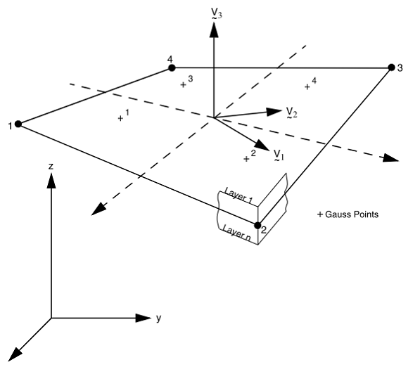
The shell elements in CivilFEM are numerically integrated through the thickness (five layers). In problems involving homogeneous materials Simpson's rule is used to perform the integration.

The layer number convention is such that layer one lies on the side of the positive normal to the shell, and the last layer is on the side of the negative normal. The normal to the element is based upon both the coordinates of the nodal positions and upon the connectivity of the element. The definition of the normal direction can be defined for five different groups of elements.

Thick shell analysis can be performed using the 4 nodes of bilinear Mindlin element. The thick shell elements have been developed so that there is no locking when used for thin shell applications.

The global coordinate system defines the nodal degrees of freedom of these elements. These elements are convenient for modeling intersecting shell structures since tying constraints at the shell intersections are not needed.

Conventional finite element implementation of Mindlin shell theory results in a constant transverse shear distribution throughout the thickness of the element.

An extension has been made for the thick shells such that a “parabolic” distribution of the transverse shear stress is obtained. In subsequent versions, a more “parabolic” distribution of transverse shear can be used. For thick shells the new formulation is approximate since it is derived by assuming that the stresses in two perpendicular directions are uncoupled.

section type	Reference
Doubly curved	4 nodes quadrilateral 3 node degenerated triangle

Shell finite elements have six degrees of freedom:

u_x = Global Cartesian x-direction displacement

u_y = Global Cartesian y-direction displacement

u_z = Global Cartesian z-direction displacement

_x = Rotation about global x-direction

_y = Rotation about global y-direction

_z = Rotation about global z-direction

Bilinear thick-shell element (4 node)

This is a four-node thick shell element (that has transverse shear effects) with global displacements and rotations as degrees of freedom. Bilinear interpolation is used to represent coordinates, displacements and the rotations. The membrane strains are obtained from the displacement field; the curvatures from the rotation field. The transverse shear strains are calculated at the middle of the edges and interpolated to the integration points. In this way, a very efficient and simple element is obtained which exhibits correctbehavior in the limiting case of thin shells. This element can be used in curved shell analysis as well as in analysis of complicated plate structures. For the latter case, the element can easily be to use since connections between intersecting plates can be modeled without tying.

Due to its simple formulation when compared to the standard higher-order shell elements, it is less expensive and, therefore, very attractive in nonlinear analysis. However the element is not very sensitive to distortion, particularly if the corner nodes lie in the same plane. All constitutive relations can be used in this element.

Generally four nodes are used per element however, the element can be collapsed into a triangle.

Each elements are defined geometrically by the (x, y, z) coordinates of the four corner nodes. Due to bilinear interpolation, the surface forms a hyperbolic paraboloid which is then allowed to be degenerated into a plate.

Bilinear thickness variation is allowed in the plane of the element.

The stress output is given with respect to local orthogonal surface directions- V_1, V₂, and V₃-for which each integration point is defined in the following way:

A set of base vector tangents to the surface is first created. The first t₁ is tangent to the first isoparametric coordinate direction. The second t₂ is tangent to the second isoparametric coordinate direction. In simple cases of a rectangular element, t₁ would be in the direction from node 1 to node 2 and t₂would be in the direction from node 2 to node 3.

In nontrivial (non-rectangular) cases, a new set of vectors

and

would be created which are orthogonal projections of t₁ and t₂. The normal is then formed as

Note that the vector

would be in the same general direction as

Therefore

There is a higher order element, an eight-node thick shell element (including transverse shear effects) with global displacements and rotations as degrees of freedom.

Second-order interpolation is used for coordinates, displacements and rotations. The membrane strains are obtained from the displacement field; the curvatures from the rotation field. The transverse shear strains are calculated at ten special points and interpolated to the integration points. In this way, this element behaves correctly in the limiting case of thin shells. The element can be degenerated to a triangle by collapsing one of the sides.

The stiffness of this quadratic element is formed using four-point Gaussian integration. The mass matrix of this element is formed using nine-point Gaussian integration.

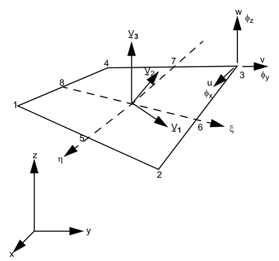
Bilinear thick-shell element (8 node)

This higher order element is an eight-node thick shell element with global displacements and rotations as degrees of freedom.

The element is defined geometrically by the (x, y, z) coordinates of the four corner nodes and four midside nodes. The element thickness is specified in the structural element. The stress output is given with respect to local orthogonal surface directions

and for which each integration point is defined in the following way:

4. Solid finite elements

CivilFEM contains solid elements that can be used to model plane stress, plane strain, axisymmetric and three-dimensional solids. These elements have only displacement degrees of freedom. As a result, solid elements are not efficient for modeling thin structures dominated by bending. Either beam or shell finite elements should be used in these cases.

The solid elements that are available in CivilFEM have either linear or quadratic interpolation functions.

They include:

Solid type	Reference
Plane stress	4 node quadrilateral
	3 node triangle
Plane strain	4 node quadrilateral
	3 node triangle
Axisymmetric	4 node quadrilateral
	3 node triangle
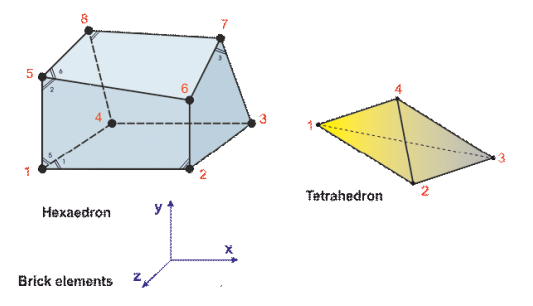
3D Solid	8 node hexaedral
	20 node hexaedral
	4 node tetrahedron
	10 node tetrahedron

In general, the elements in CivilFEM use a full-integration procedure. Some elements use reduced integration. The lower-order reduced integration elements include an hourglass stabilization procedure to eliminate the singular modes.

The 8-and 20-node solid brick elements can be degenerated into wedges and tetrahedra by collapsing the appropriate corner and midside nodes. The number of nodes per element is not reduced for degenerated elements. The same node number is used repeatedly for collapsed sides or faces. When degenerating incompressible elements, exercise caution to ensure that a proper number of Lagrange multipliers remain. User is advised to use the higher-order triangular or tetrahedron elements wherever possible, as opposed to using collapsed quadrilaterals and hexahedra.

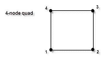
Four-node plane stress quadrilateral

This element is a four-node, isoparametric, arbitrary quadrilateral written for plane stress applications. As this element uses bilinear interpolation functions, the strains tend to be constant throughout the element. This results in a poor representation of shear behavior . The shear (or bending) characteristics can be improved by using alternative interpolation functions.

This element is preferred over higher-order elements when used in a contact analysis.

The stiffness of this element is formed using four-point Gaussian integration.

All constitutive models can be used with this element.

To improve the bending characteristics of the element, the interpolation functions are modified for the assumed strain formulation.

Degrees of Freedom:

1 = u (displacement in the global x direction)

2 = v (displacement in the global y direction)

Three-node plane stress triangle

This element is a three-node, isoparametric, triangular element written for plane stress applications. This element uses bilinear interpolation functions. The stresses are constant throughout the element. This results in a poor representation of shear behavior .

The stiffness of this element is formed using one point integration at the centroid. The mass matrix of this element is formed using four-point Gaussian integration.

Degrees of Freedom

1 = u (displacement in the global x direction)

2 = v (displacement in the global y direction)

Four-node plane strain quadrilateral

This element is a four-node, isoparametric, arbitrary quadrilateral written for plane strain applications. As this element uses bilinear interpolation functions, the strains tend to be constant throughout the element. This results in a poor representation of shear behavior . The shear (or bending) characteristics can be improved by using alternative interpolation functions.

This element is preferred over higher-order elements when used in a contact analysis.

The stiffness of this element is formed using four-point Gaussian integration.

Degrees of Freedom

1 = u (displacement in the global x direction)

2 = v (displacement in the global y direction)

Three-node plane strain triangle

This element is a three-node, isoparametric, triangular element written for plane strain applications. This element uses bilinear interpolation functions. The strains are constant throughout the element. This results in a poor representation of shear behavior.

The stiffness of this element is formed using one point integration at the centroid. The mass matrix of this element is formed using four-point Gaussian integration.

Degrees of Freedom

1 = u (displacement in the global x direction)

2 = v (displacement in the global y direction

Four-node axisymmetric quadrilateral

10 is a four-node, isoparametric, arbitrary quadrilateral written for axisymmetric applications. As this element uses bilinear interpolation functions, the strains tend to be constant throughout the element. This results in a poor representation of shear behavior .

This element is preferred over higher-order elements when used in a contact analysis.

The stiffness of this element is formed using four-point Gaussian integration.

Degrees of Freedom

1 = u (displacement in the global z-direction)

2 = v (displacement in the global r-direction)

Three-node axisymmetric triangle

This element is a three-node, isoparametric, triangular element. It is written for axisymmetric applications and uses bilinear interpolation functions. The strains are constant throughout the element and this results in a poor representation of shear behavior.

The stiffness of this element is formed using one-point integration at the centroid. The mass matrix of this element is formed using four-point Gaussian integration.

Degrees of Freedom:

1 = u = axial (parallel to symmetry axis)

2 = v = radial (normal to symmetry axis)

Three-dimensional arbitrarily distorted brick

This element is an eight-node, isoparametric, arbitrary hexahedral. As this element uses trilinear interpolation functions, the strains tend to be constant throughout the element. This results in a poor representation of shear behavior. The shear (or bending) characteristics can be improved by using alternative interpolation functions.

This element is preferred over higher-order elements when used in a contact analysis.

The stiffness of this element is formed using eight-point Gaussian integration.

This element can be used for all constitutive relations.

Three global degrees of freedom u, v, and w per node.

Three-dimensional 20-node brick

This element is a 20-node, isoparametric, arbitrary hexahedral. This element uses triquadratic interpolation functions to represent the coordinates and displacements; hence, the strains have a linear variation. This allows for an accurate representation of the strain fields in elastic analyses.

The stiffness of this element is formed using 27-point Gaussian integration.

This element can be used for all constitutive relations.

Three global degrees of freedom, u, v and w.

Reduction to Wedge or Tetrahedron: by simply repeating node numbers on the same spatial position, the element can be reduced as far as a tetrahedron. 10-node tetrahedron is preferred in this case.

Three global degrees of freedom, u, v and w.

Three-dimensional four-node tetrahedron

This element is a linear isoparametric three-dimensional tetrahedron. As this element uses linear interpolation functions, the strains are constant throughout the element. The element is integrated numerically using one point at the centroid of the element. This results in a poor representation of shear behavior. A fine mesh is required to obtain an accurate solution. This element should only be used for linear elasticity. The higher-order element is more accurate, especially for nonlinear problems.

This element can be used for all constitutive relations.

Three global degrees of freedom, u, v, and w.

Three-dimensional ten-node tetrahedron

This element is a second-order isoparametric three-dimensional tetrahedron. Each edge forms a parabola so that four nodes define the corners of the element and a further six nodes define the position of the “midpoint” of each edge.

This allows for an accurate representation of the strain field in elastic analyses.

The stiffness of this element is formed using four-point integration. The mass matrix of this element is formed using sixteen-point Gaussian integration.

The element is integrated numerically using four points (Gaussian quadrature).

Three global degrees of freedom, u, v, and w.