20.1                 Introduction

The aim of this module is to provide a utility that allows the study of the prestressing effects in concrete structures.

CivilFEM calculates post-tensioned and pre-tensioned adherent inner tendons.

The tendons definition is possible to be carried out by an interactive and graphical way using the tendon editor with multiple options to generate, modify, copy, delete and so on.

The prestress losses are calculated and therefore the forces and stresses distributions throughout each one of the tendons are obtained.

Utilities for the transference, to the finite element model, of the prestressing forces have been implemented, either for beam, shell or solid models, apart from tapered beam elements, which these utilities are not supported.

The module also provides the possibility of checking by code cracking, axial load plus biaxial bending, shear and torsion.

Throughout the chapter principles and formulation followed in each operation are exposed.

 

20.2                 Support Beam

All the necessary data for the prestressed structure analysis are condensed into the so-called “support beam”.

The definition of the support beam is done once the finite element model is created (see ~SBBMDEF, ~SBSMDEF,  ~SBSMMDF and ~PCCTMDF commands).

The support beam is defined by a series of segments delimited by cuts. Therefore, the support beam will have N segments and N+1 cuts.

If the support beam comes from a beam element model, there will be one segment associated to each element and there will be as many cuts as nodes in the model. If the support beam comes from a solid element model, the cuts will correspond to the solid sections defined by user.

Therefore, the cuts contain the data related to the location and orientation of the cross sections and the segments contain the information related to the geometry of the model.

20.2.1                  Coordinate Systems

The support beam is captured in the active coordinate system. If the capture process is done in several phases, the coordinate system used will be the initial one, this is to say, the one used at the beginning of the capture of the support beam.

In order to detect the vertical direction of the model, and correctly understand the plan and elevation views, it is necessary that the active coordinate system at the moment of capture of the support beam follows these guide lines:

• The vertical direction axis (gravity direction) is the Y axis.
• It is recommended that the X axis follows the predominant direction of the prestressing tendons that will be defined.

If the support beam comes from a solid model, it will be defined by solid sections. These sections have an associated coordinate system (the one used for its definition), with the X axis perpendicular to the section. The positive direction of the X axis should be oriented towards the advancing direction of the support beam (from the first to the last cut).

For beam element models, the offset of the section must be set (in the beam & shell properties) at the section axis origin.

 

20.3                 Tendons Editor

20.3.1                  Introduction

The CivilFEM tendons editor allows to graphically define the layout geometry and the mechanical properties of the multiple prestressing tendons as well as to calculate the prestressing losses of each one of them.

The tendons are placed in the so-called support beam (the tendons lean on the support beam), therefore it must de defined before editing the tendons.

20.3.2                  Prestressing cables layout

20.3.2.1                   Introduction

For CivilFEM, the prestressing layout corresponds to the geometric and mechanical definition of a tendon.

For designing prestressing tendons layout by hand-calculation, the cable layout is usually represented as a set of vertical axis parabolas and straight segments that are tangents one to another.

The reasons for choosing vertical axis parabolas to represent the prestressing cables layout are the following:

-          The hand-calculation is done over 2D layouts (contained in a plane), assuming that the beam axis is parallel to the X-axis and that the slopes are smooth. In these conditions, the parabola comes close to the catenary, which is the curve that really describes the shape of a flexible cable supported at two points.

-          The calculation of the vertical deviation forces in parabolas is trivial since the curvature can come close to the second derivate with respect to X and, consequently, to a constant. It leads to a constant stress (for a constant cable stress) as the cable deviation force. More exactly, the vertical deviation force of a cable that follows a curve is proportional to its second derivate and to the cable stress and, therefore, in a parabola it is exactly a constant.

-          The tangent adjustment (between two adjacent parabolas or between a parabola and a straight segment) is solved with a simple linear equation system.

Nevertheless, CivilFEM does not use vertical axis parabolas to represent the prestressing cables layout but it uses second order Bezier curves.

The second order Bezier curves have notable advantages with respect to the straight segments and to the vertical axis parabolas. The most important could be the following:

-          A second order Bezier curve is able to link any two points entering in both points with prefixed tangents, which allows for a local control of tangencies and depths.

-          The second order Bezier curves can represent 3D layouts without problem, and with the same equations they can be used to represent them in 2D.

-          The shape of a prestress casing in the space is very close to a Bezier curve. It cannot be approximated by a vertical axis parabola, since the space does not have a specific axis system.

-          The vertical axis parabola is a particular case of a second order Bezier curve. The same thing logically happens for the straight segments.

-          The Bezier curves are much more efficient than the explicit.

-          Bezier curves are widely used in drawing packages (CAD software) and in some cases are refered as splines. Although, a spline is formally a succession of Bezier curves with some continuity level of function, derivate and second derivate.

Figure 20.3.1 3D Splines generation

20.3.2.2                   Geometric definition of a cable layout

In CivilFEM, two different shapes define a tendon: one defines the plan view and the other the elevation view.

Each one of these shapes is defined by a succession of second order Bezier curves.

In 2D problems, the user only has to define the layout in elevation view, adopting the trivial configuration (Z=0) for the layout in plan view.

The layout in elevation view is the one that normally really controls the structural prestressing effect. Simultaneously, the layout in plan view allows to correctly locate the different tendons through the structure in the case of 3D models, as well as positioning the tendons inside the sections.

20.3.2.3                   Control points of the layout

The cable geometry is defined by a sequence of control points among which the consecutive curves that define the layout are interpolated, taking into account some tangency and degree conditions defined by the user.

The control points of the layout are referenced to the local coordinate systems of the support beam cuts. Each layout point should be contained in the YZ plane of one of the local coordinate systems of the sections (cuts).

There are two groups of control points: the control points of the elevation view (see ~PCEPDEF command) and the control points of the plan view (see ~PCPPDEF command) that are independent.

20.3.3                  Layout in elevation view

The user defines the layout in elevation view cast over a plane that can be considered as the development of an imaginary surface, warped in the space, that contains the local Y axis of the cross section cuts. 

The layout in elevation view is defined by a sequence of second order Bezier curves, each one of them connecting two consecutive control points. The coordinates of the control points and the established tangency conditions define the curve.

In the elevation view, the user can define or modify the number and locations of the control points as well as their slope.

The user can, as normal, directly introduce the Ypt coordinate and the Ysl slope for a specific point. Anyway, the usual way of handling these data will be by an indirect reference to them, as a result of the conditions imposed to the layout.

20.3.4                  Layout in plan view

The layout in plan view is made by a sequence of second order Bezier curves that connect successive control points.

It works in the same way as the layout in elevation view.

20.3.5                  Inflection points

There is no second order Bezier curve that can be drawn between two points with parallel tangents, except for the singular case of a straight line.

In order to resolve this geometrical situation without having to insert an intermediate point with its associated cut in the support beam, CivilFEM introduces the concept of Inflection Point associated to a tendon point.

The curve between the two points with parallel tangents (not necessarily horizontal) will be broken down into two Bezier curves, with the joint point between them located at a certain distance from the first point. This distance is defined as a property of the point (just as the slope).

 

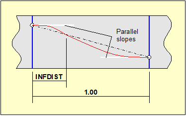
Figure 20.3.2 Inflection points

The curves created will be vertical axis parabolas. Therefore the tangential point will be located on the straight line that connects the two points.

 

20.4                 Prestressing Losses

20.4.1                  Introduction

CivilFEM takes into account the post-tensioned internal adherent reinforcement and the pretensioned reinforcement.

Prestressing with post-tensioned reinforcement is done alter the concrete is built. Reinforcement goes through ducts which are left inside concrete. When concrete has achieved its required strength, the prestressing process is done.

For pretensioned reinforcement, the tendons are prestressed before concrete is placed and are anchored to provisional restraining elements. When concrete has achieved its required strength, the reinforcement is freed from the restrains, and due to the adherence between the reinforcement and concrete, the prestressing action is transferred to the concrete.

 

20.4.2                  Immediate losses

The immediate losses of prestress occur once the prestressing force is applied, after the concrete has been placed and cured, and when the tendons are anchored.

Its value for pre-tensioned members is the following:

Where:

DP₁: Losses due to steel relaxation before transfer and due to heating.

DP₂: Losses due to thermal steel expansion.

DP₄: Losses due to the slippage of strands in the anchorages.

DP₅: Losses due to elastic shortening of concrete member.

For post-tensioned members, its value is the following:

Where:

DP₃: Losses due to friction through the prestressing duct.

DP₄: Losses due to the slippage of strands in the anchorages.

DP₅: Losses due to elastic shortening of concrete member.

20.4.2.1                   Losses due to steel relaxation before transfer and due to heating. (DP₁)

This loss is provided by the manufacturer. If it is not provided, CivilFEM calculates it by supposing its value is equal to the long-term steel relaxation losses for a time corresponding to 10⁶ hours and at environment temperature. That is, the total steel relaxation losses are twice the long-term steel relaxation losses (DP₈).

20.4.2.2                   Losses due to thermal steel expansion (DP₂)

Thermal steel expansion losses due to heating process are given by the following equation:

Where:

K	Thermal reduction factor. By default it is equal to 0.9 (Value proposed by CEB-FIB Code)
a	Thermal expansion coefficient of the tendon steel.
Ep	Elasticity module of the tendon steel.
Tc	Heating temperature at production process.
Ta	Environment temperature at production process.

20.4.2.3                   Losses due to friction (DP₃)

The prestressing friction losses between a given point, normally the anchorage device, and other point located at a distance x from the first one is given by the following equation:

Where:

P0	Initial tendon prestressing force.
m	Friction coefficient between the tendons and their casing.
a	Sum of the angular displacements, measured in radians, over a distance x. The tendons layout can be a warping curve, evaluating a in the space.
K	Unintentional angular displacement per unit length.
X	Real distance through the tendon between the considered section and the operative anchorage device.

 

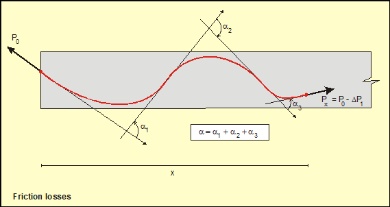
Figure 20.4.1 Losses due to friction

The m and K values are defined in the material properties associated to the tendon.

20.4.2.4                   Losses due to slippage of strands in the anchorages (DP₄)

These losses take place when there is a drive-in of the tendons at the anchorage, during the operation of anchoring after tensing, and of the deformation of the anchorage.

The anchorage slip value is established in the material associated to the corresponding tendon.

Due to the friction, the value of this loss depends on the distance to the anchorage device.

The shortening of the cable produces a relaxation that is developed through an extension w in plan view in such way that the following condition is verified:

Or

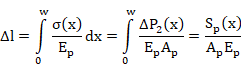
The problem is solved if found the extension w for which the value of the shadowed area of the bellow figure, divided by the product E_p ^.A_p, coincides with the elongation Dl = a, of slip anchorage.

 

 Figure 20.4.2 Losses due slip anchorage

CivilFEM contemplates the possibility of partial tensing and releasing. The losses due to the releasing operation are calculated in the same way as for the anchorage slip losses, taking, in this case, the stress increment as known datum.

The slippage of strands in the anchorages for pre-tensioned members produces a constant loss in the length of the tendon due to absence of the friction. This value is given by the following equation:

Where:

a	Anchorage slip.
L	Length of the tendon.
EP	Elasticity module of the tendon steel.
AP	Area of tendon.

20.4.2.5                   Losses due to elastic shortening of concrete (DP₅)

CivilFEM allows for the step by step tensing of the tendons. It means the possibility of prestressing one or more tendons at the same time, when other tendons have already been anchored.

Tensing a tendon causes some instantaneous deformations in the concrete member and, therefore, it causes losses in the previously anchored tendons.

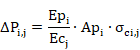
The deformation caused by prestressing a j tendon in the concrete member adjacent to the already anchored tendon i and in the tendon itself has the following value:

Therefore, the loss in the anchored i tendon force, caused by the j tendon prestressing, will be:

where:

	Area of tendon i.
	Elasticity module of steel of tendon i.

Therefore

 

	Concrete elasticity module at the moment of prestressing the tendon j.
	Stress in the concrete adjacent to tendon i. It’s calculated from the acting prestressing force (initial prestressing force less the friction and anchorage slip losses) on the considered point. The self-weight and other permanent actions are not taken into account for this stress calculation.

 

For pre-tensioned members, the elastic shortening of concrete is produced when the tendons are casted off the anchorage. Therefore, the difference to the post-tensioned is that all the tendons are released at the same time.

 

20.4.3                  Long-term losses

The long-term losses are time-dependent losses that occur after the end of the last prestressing operation.

The time-dependent losses are due to the following reasons:

-          Losses due to concrete shrinkage.

-          Losses due to concrete creep.

-          Losses due to steel relaxation.

20.4.3.1                   Losses due concrete shrinkage (DP₄)

For a given concrete age t, these losses are calculated according to the bellow expression:

Where e_sr (t, t₀) is the estimated shrinkage strain (t₀ is the concrete age at the initial loading of the concrete). A constant value is taken for this parameter, which is supplied by the user in the material properties definition.

20.4.3.2                   Losses due concrete creep (DP₅)

These losses are calculated according to the bellow expression:

where:

scp0	Stress in the concrete adjacent to the tendons, due to prestress.
scg	Stress in the concrete adjacent to the tendons, due to the permanent actions.
n	Equivalence coefficient Ep/Ec.
j (t, t0)	Creep coefficient for a concrete age t and a concrete age t0 at the initial loading of concrete.

 

The coefficient j (t, t₀) is taken as a constant that should be defined by the user in the material properties definition.

The value of stress in the concrete due to prestress and to the permanent loads ((s_cg (x) + s_cp0 (x)) should be introduced by the user when defining the tendons. It is possible to define a different value for each considered section. By default it is equal to 5 N/mm².

20.4.3.3                   Losses due steel relaxation (DP₆)

These losses are calculated from the following equation:

where:

P(x)	Force in the tendon after the immediate losses have occurred.
rrl (t, sp , fpk)	Relaxation function that depends on the active code.

a)    EUROCODE Nº 2

The value of the relaxation coefficient in each point of the tendon is obtained by interpolating for the stress value and the considered time.

The stress is interpolated from the relaxation values, introduced in the material properties, corresponding to 60%, 70% and 80% of the initial stress with respect to the characteristic tensile strength and to the 1000 hours.

For stress values less than 60%, the interpolation is done considering that the relaxation is null for values under 50%.

The time is interpolated considering that the evolution of the losses between 0 and 1000 hours is the following (table 4.5 of Eurocode 2, ENV 1992-1-1:1992):

Table 20.4.1 Relationship between relaxation losses and time up to 1000 hours

Time in hours	1	5	20	100	200	500	1000
Relaxation losses as % of losses after 1000 hours	15	25	35	55	65	85	100

The long-term losses are considered to take place for a time corresponding to 10⁶ hours and have a value of LtRat times the relaxation losses at 1000 hours. The LtRat value is defined in the material properties ( by default LtRat = 3).

The calculation of a time exceeding 1000 hours is done by interpolating between this value and the one corresponding to 10⁶ hours.

 

b)    ACI-318 codes

The relaxation losses are calculated by means of the expression:

where:

t	time in hours in which the losses are evaluated.
fpi	tendon stresses after discounting the instantaneous losses.
fpy	specified yield strength of presstressing tendons.
RlCf1	Coefficient that depends on the prestressing steel type StTp = 0 (Low-relaxation) RlCf1 = 45 StTp = 1 (stress-relieved) RlCf1 = 10
RlCf2	Coefficient (default value = 1.0)

Prestressing losses are not calculated for ACI 359 code.

c)    EHE

The relaxation coefficient is calculated as:

Where k₁ and k₂ are coefficients that depend on the steel type and on the initial stress. The coefficients k₁ and k₂ are calculated from the material relaxation data corresponding to 60%, 70% and 80% of the stress with respect to the characteristic tensile strength and to the ages introduced by the user. Once these coefficients are obtained, a linear interpolation is done for the given stress, assuming the relaxation corresponding to 50% of the stress with respect to the characteristic tensile strength as null.

20.4.3.4                   Approximate calculation procedures

The long-term prestressing losses, as previously stated, suppose the maintenance of constant stress in tendons, which is incompatible with the existence of the long-term losses.

Depending on the long-term losses magnitude, compared with the total prestress force, the explained calculation will be more or less accurate.

The different codes supply some simplified formulations in order to take into account all the multiple phenomena that take place in the long-term losses generation.

A more accurate calculation requires a step-by-step integration process in a time coupled with the structural analysis.

a)    EUROCODE Nº 2

where:

	Variation of stress in the tendons due to creep, shrinkage and relaxation at location x at time t.
	Shrinkage strain. It is taken as a constant and its value is supplied in the material properties
	Equivalence coefficient = Ep/Ec.
Ep	Elasticity modulus for the prestressing steel.
EC	Elasticity modulus for the concrete at the age at which the long-term losses are evaluated.
	Creep coefficient. It is taken as a constant and its value is supplied  in the material properties
	Stress in the concrete adjacent to the tendons, due to prestress and permanent loads. It is defined by user when creating the tendons.
AP	Area of all prestressing tendons.
AC	Area of the concrete section.
IC	Moment of inertia of concrete section.
ZPC	Distance between the center of gravity of the concrete section and the tendons.
	Ageing coefficient. It is introduced as an argument in the ~PCLOSS command for calculating the prestressing losses (default value c= 0.8).
	Variation of stress in the tendons at location x due to relaxation.

 

b)    EHE

The EHE code allows evaluating the long-term losses according to the following simplified expression:

where:

	Shrinkage strain. It’s taken as a constant and its value is supplied in the material properties
	Equivalence coefficient = Ep/Ec.
Ep	Elasticity modulus for the prestressing steel.
EC	Elasticity modulus for concrete at the age at which the long-term losses are evaluated.
	Creep coefficient. It’s taken as a constant and its value is supplied in the material properties
	Stress in the concrete adjacent to the tendons, due to prestress and permanent loads. It is defined by user when creating the tendons.
	Variation of stress in the tendons due to relaxation.
AP	Area of all prestressing tendons.
AC	Area of the concrete section.
IC	Moment of inertia of concrete section.
yP	Distance between the center of gravity of the concrete section and the tendons.
	Ageing coefficient. It is introduced as an argument in the ~PCLOSS command for calculating the prestressing losses (default value = 0.8).

 

c)     Dischinger-Birkenmaier solution

where:

	Losses due to concrete shrinkage.
	Losses due to concrete creep.
Pki	Prestress action after all the immediate losses have occurred.
	Axial force in concrete without taking into account the prestress. It is taken as N=0.
EC	Elasticity modulus for concrete at the age at which the long-term losses are evaluated.
An	Area of the concrete section.
AP	Area of all prestressing tendons.
EP	Elasticity modulus for the prestressing steel.
	Shrinkage strain. It is taken as a constant and its value is supplied in the material properties
	Creep coefficient. It is taken as a constant and its value is supplied in the material properties

 

The obtained losses due to concrete shrinkage and creep are stored separately, sharing them at the same proportions as if the calculation was done following the Eurocode 2 approximate procedure.  

The losses due to steel relaxation are calculated as it was shown in the corresponding section.

 

20.5                 2D Interaction Diagram

20.5.1                  Pivots Diagram

The interaction diagram is a surface in space (F,M) that contains the forces and moments corresponding to the section’s ultimate strength states. In CivilFEM the ultimate strength states are determined through the pivots diagram.

 

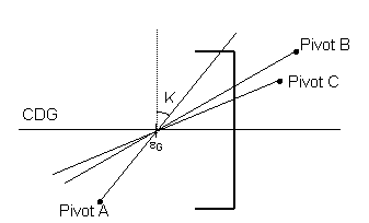
Figure 20.5.1 Pivot Diagram

A pivot is a strain limit associated with a material and its position in the section. If the strain in a section’s pivot exceeds the limit marked for that pivot, the section is cracked. Pivots delimit thus the positions of the strain plane. So, in an ultimate strength state, the strain plane supports at least one pivot of the section.

In CivilFEM pivots are defined as material properties and these properties (pivots) are extrapolated to all the section’s points, taken into account the material of each point. So, the pivots considered for the section’s strain plane determination, correspond to the following material properties (see chapter 3 of the Theory Manual):

 

            A Pivot =        EPSmax. Maximum allowable strain in tension at any point of the section (the maximum of the maximum strains allowable in each point of the section in case there are different materials in the section).

            B Pivot =        EPSmin. Maximum allowable strain in compression at any point of the section(the maximum of the maximum strains allowable in each point of the section).

            C Pivot =        EPSint. Maximum allowable strain in compression at section’s interior points.

 

For the determination of the strains plane the Navier’s hypothesis is assumed. The strain’s plane determination is defined according to the following equation:

 

where:

e (y)	Strain of a section point in function of the Y, Z axes of the section.
eg	Strain in the origin of the section (center of gravity)
K	Curvature

20.5.2                  Prestressing steel strains

In the calculation of total prestressing steel strains, apart form the strain produced in the corresponding ultimate state deformation plane fiber, the prestressing strain and the decompression strain are also considered:

 

Where:

	Concrete decompression strain at the considered reinforce level
	Prestressing steel strain due to the prestressed action in the considered phase, considering the losses that have taken place.

The strain decompression calculation is carry out taking into account the initial prestressed on the effective section and the long term losses on the homogenize section. 

20.5.3                  Diagram construction process

 To determine the strains plane (ultimate strength plane) of the section. e_g and q are used as independent variables. The process is composed of the following steps:

1. Pivots calculation for each the cross section points are based on the associated material, its position within the cross section and the prestressed in case of the prestressing steel.
2. From the total pivots number  a deformation planes sweeping is made passing through some of the pivots (without going through any of them).
3. Each one of the strain planes (ultimate strength plane) correspond with a curvature and a strain in the section’s center of gravity and determine the deformation corresponding to each of the section points e(y).
4. From the e(y) strain and the prestressing steel pre-deformations, the stress corresponding to each point of the section (sp) is calculated entering in the material stress-strain diagram of each point. This way, the stress distribution inside the section is determined.

 

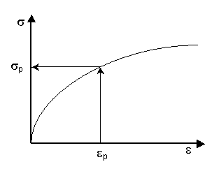
Figure 20.5.2 Stress determination in a point

5. So, as the stress distribution is known, the corresponding ultimate forces and moments (Fu, Mu), are obtained by the summation of stresses on each one of the sections point multiplied by its corresponding weight according to the considered flexion axis.    

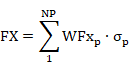
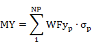
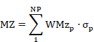
Where:

NP	Number of points of the section.
WFX, WMY, WMZ	Weights of each section points.

The contribution of the prestressing steel is added to these forces and moments.

 

6. From the ultimate obtained  forces and moments a distribution of those is made to obtain the closed curve that defines the diagram.

 

20.5.4                  Determination of the diagram center

Reinforce concrete interaction diagrams left the coordinates origin on its interior, but in the  prestressed concrete sections the origin may be a point belonging to the surface or even a point outside the diagram. In this situation the section is cracked for null forces and moments.

To avoid these singular situations, in the cases where the origin is a  point outside the diagram, CivilFEM changes the axes, placing the origin of the coordinate system in the geometric center of the diagram.

In this case, the calculation of the safety criterion is made according to the new coordinates origin instead of the real origin.

 

20.6                 Axial Load and Biaxial Bending Checking

The procedure used, in the axial load and biaxial bending checking of prestressed cross sections, is based on the 2D interaction diagram, of the analyzed cross section, construction.

20.6.1                  Calculation Hypothesis

·         Checking is made to axial load and biaxial bending, according to one of the section local axis (Y o Z) requested for the user, without taking into account the moment corresponding to the other direction.

·         Checking is only made to comply with the section’s strength requirements, thus ignoring the requirements related to the serviceability conditions, minimum reinforcement amounts or dispositions for each code, environment and structural typology.

·         It is assumed always as valid the Navier’s hypothesis, according to which the deformed section stays plain. Longitudinal strain of concrete and steel is proportional to the distance to the neutral axis.

20.6.2                  Calculation Process

Checking of elements in axial force and biaxial bending is made in the following steps: 

1.     Obtaining the acting forces and moments of the section (FXd, MYd, MZd) of which the primary prestressing forces and moments are subtracted (Fxiso, Myiso or Mziso). The acting forces and moments are obtained, after making a calculation, directly from the CivilFEM results file (file .RCV).

2.     Construction of the interaction diagram of the section (see construction process in the previous section). From the diagram, that contains all the ultimate pairs of forces and moments (Fu, Mu) of the cross section, the ultimate strain state homothetic to the acting point (point P) with respect to the diagram center is determined (see the previous section for the determination of the diagram center).

 

Figure 20.6.1 Determination of the homothetic strain state

3.     Obtaining the strength criterion of the section. This criterion is defined as the ratio between the distance of the “center” of the diagram (point A of the figure) to the point which represents the acting forces and moments (point P of the figure) and to the point which represents the homothetic ultimate forces and moments (point B).

If the criterion is less than 1.00, in such a way that the forces and moments acting on the section are inferior to its ultimate strength, the section is safety. On the contrary (criterion higher than 1.00), the section will be considered as no valid.

20.6.3                  Important considerations

-          The axial load and biaxial bending checking requires, in addition to the total forces and moments, the primary ones. These forces and moments are calculated and are stored in the results file along with the totals. The primary prestressing forces and moments are not possible to be defined as ‘targets’, but they are combined as concomitants.

-          In the axial load and biaxial bending calculations it is also necessary to know the parameters that define the prestressing action (support beam, tendons definition, prestressing losses...). These parameters are written within the corresponding ‘load step’ results block.

-          Therefore, the load step combinations of axial load and biaxial bending calculations, must contain a single load step to which the prestress is applied. The prestressing data of this single load step will be written in the combined state.

-          Two or more prestressing loads can be combined together if they have the same definition (active tendons, losses parameters, etc.). If the prestressing actions have different topology, it is recommended to use them independently, as different combinations, and create envelopes with the results.

 

20.7                 Cracking Checking

The prestressed cross section cracking checking is available in the current CivilFEM version for the following codes:

-          Eurocode 2

-          ACI 318

-          EHE

-          ITER Design Code

The checking consists of the verification of the decompression state or the crack width calculation. This last one is made taking into account the bending according to the local cross section axis, as a user request, and the bending moment in the perpendicular direction.

The crack opening calculation is performed as a reinforce concrete cross section considering the prestressed action like a external action and existing the prestressing steel in the cross section.

The hypotheses, used formulation and obtained results in each code can be studied in the reinforced concrete cross sections cracking.

In the case of bridge cross sections (slab or box) the code properties necessary for the checking are not calculate automatically, reason why the user must be the one that defines them (see ~SECMDF command).

The ~CHKPRS checks according to the cracking prestressed cross sections and its arguments are the same as  reinforced concrete cross sections (~CHKCON command).

Regarding to the checking results, they are the same as the reinforced concrete (see   ~PLLSPRS command).

 

20.8                 Free Tendons (Independent from Support Beam)

20.8.1                  Introduction

It is possible to define the tendons as a 3D curve in space, without the creation of a support beam.

This allows its application on any model, meshed with 3D solid elements.

Since there is no support beam, CivilFEM will not be able to capture the behaviour of the model and the interaction of it with the tendons, so the prestressing losses will not be fully calculated.

The decomposition of forces and moments into primary and secondary due to the prestressing actions cannot be done either.

20.8.2                  Tendon definition

Tendon definition is carried out introducing the coordinates in the space of the points forming the tendon, as well as the value of the tension force at these points. This capability is accessible through the following group of commands:

~PCCBST, IdCable

~PCCBPA, x, y, z, T, p1, p2, p3, q1, q2, q3

_…

~PCCBEND

Where:

IdCable	Cable identification number.
X, Y, Z	Point coordinates in the space.
T	Point stress (force units).
p1, p2, p3	Tangent vector to the point’s previous segment.
q1, q2, q3	Tangent vector to the point’s subsequent segment.

20.8.3                  Introduction of the tendons’ action over the structure

Loads transference is done by using the ~TENLD command which loads the model with the desired tendons, without deleting any previously defined loads.