17-A.1               Introduction

The Geotechnical and Foundations Module was created to provide a powerful tool to assist civil engineers with any type of geotechnical problem.

Within this utility, CivilFEM incorporates a geotechnical database with a wide range of tools used for analyses and calculations.  The database contains the following characteristics:

• Includes soil and rock properties not considered by ANSYS.
• Allows the user to make correlations between variables with different origins or different definitions, a very common practice in Geotechnics (for example, the correlation between the modulus of elasticity E and the standard penetration test SPT).
• Includes libraries of characteristic properties of soils and rocks as well as a vast number of correlations obtained from related literature and experience.
• Permits users to create customized libraries. 

In addition to the resources listed above, the following tools have been included:

• Slope stability analysis, including water table definition, reinforced earth, etc.
• Hoek and Brown model in order to simulate the behavior of rock foundations, and Mohr-Coulomb and Cam-Clay for soils.
• Determination of the ballast module for any type of foundation.
• Generation and calculations of retaining walls.
• Seepage analysis. This tool automatically obtains the saturation line and solves the seepage problem through a porous media.
• Tunnel models.
• Initial stresses for soils.
• Calculation and application of earth pressures on structures.

17-A.2      Definition of Layered Soils

The layered soils utility is used for soils that are not directly modeled by finite elements in the model. 

The number of layers in the model is inputted by the user with a maximum value of 20 layers (see ~TERDEF command).

This utility can be used for the following applications:

• Ballast module calculation.

·         Retaining wall calculation through 2D models.

·         Earth pressures application.

·         Pile cap design.

For the applications above, the user must indicate the identification number of the soil that will be utilized; this soil must be checked to verify all of the properties have been defined to perform the desired calculation.

 

17-A.3      Ballast Module

The objective of this feature is to estimate a value for the ballast coefficient to approximate the elastic soil model (defined by E and n parameters) by means of the Winkler model (defined by its ballast module.)

Both the elastic and the Winkler model are conceptually different; therefore, it is impossible to attain an exact calculation. Furthermore, the ballast module obtained from the elastic model depends on the material, the foundation shape and the point from where it was measured. Effectively, this value will not be zero even outside the foundation.

Therefore, the most effective procedure to obtain the ballast module will consist of placing a unit load on the area enclosed by the foundation and measuring the subsidence. The amount of subsidence at each point will be the inverse of the ballast module.

The program will not only obtain the precise value of the ballast module, but also the average, maximum and minimum value.

17-A.3.1             Boussinesq

To solve for the amount of subsidence, the program uses Boussinesq’s solution as starting point. This solution focuses on the surface subsidence caused by a point load of value Q, expressed in cylindrical coordinates with the following expression:

Where:

This law presents a singularity its the origin, the point just under the load.

 

17-A.3.2             Subsidence in Foundations

For a foundation subjected to a uniform load q, according to the Boussinesq expression for any load, the subsidence in the origin is obtained from the expression:

In order to calculate the subsidence for any other point, it is necessary to perform consecutive axis displacements with the following expression:

 

17-A.3.3             Particular Cases

Particular cases have not been included in the program as only the generic case will be considered.

However, the following particular cases have been manually contrasted with the CivilFEM results and have been used as verification examples.

 

17-A.3.3.1                        Uniform Load on a Circular Surface

Considering a circular foundation with a radius, a:

• Subsidence at the center of the Shell:

      The integral calculation equals:

 

Therefore:

• At the periphery:

The integral calculation equals:

Where the relationship between the subsidence at the edge and at the center is:

• At any point:

 

For the expression where K and E are the elliptical integrals:

 

 

 

17-A.3.3.2                        Rectangular Load

For a rectangular foundation with a´b dimensions subjected to a uniform load, Steinbrenner (1936) deduced the following expression related to subsidence under a corner:

 

Where n=a/b.

In order to obtain the subsidence at any point, this rectangle is divided into four rectangles so that each rectangle all has this point in common.

17-A.3.4             Layered Soils

For earth consisting of n horizontal layers of h_i thickness, a modulus of elasticity E_i and a Poisson coefficient n_i , the subsidence calculation is done by using equivalent values of E_e and n_e. E_e is computed using a generalized form of the expression given by Thenn de Barros (1966):

 

 

 

n_e is the average of the Poisson coefficients:

17-A.3.5             Integrals

Since the generic case will be considered, the integral utilized is the following:

Where a and b are the coordinates of the foundation point for which the ballast module will be calculated and W is the area enclosed by the foundation elements.

 

The integral is defined as an integral sum of each element:

These integrals are numerically solved by using Gauss´ points. However, a problem exists for those elements that contain the point P (a,b). For this point, the function below will present a singularity:

Because the integral for these elements does not produce a finite solution, it will be solved in polar coordinates. Consequently, the element is then divided into triangles with the point P (a,b) as a common vertex:  

Figure 17-A.3‑1 Triangle Division of an Element

 

When the variables change to polar coordinates, the integral is the following:

For each triangle:

 

17-A.3.6             Relationship Between the Ballast Module and the EFS

The Elastic Foundation Stiffness (EFS) is the stiffness of the earth, relating to vertical loads. Therefore, the EFS is the ballast module.

 

17-A.4               Retaining Walls 1 ½ D

17-A.4.1             Introduction

This capability calculates data values for retaining walls through 2D non-linear and evolutive finite element models for the different excavation levels. The retaining wall will be modeled using beam elements and its interaction with soil will be represented by beams and contact elements.

The material of the retaining wall may be steel or concrete. Furthermore, the wall can be considered as a non-linear structure and the user may apply the non-linear concrete module to perform the calculations.

The retaining wall must be vertical for these calculations, but it is possible to consider a surface load over an inclined slope of earth, as shown in the following figure.

Figure 17-A.4‑1 Schematic view of the problem

17-A.4.2             Earth

Modeling earth with different soil layers is performed by using the ~TERDEF command. With this command the user can define all of the material properties required for the earth pressure calculation.

17-A.4.3             Modeling

The retaining wall is modeled with 2D beam elements; all boundary conditions and actions independent of the actions from the earth pressure and the water table must be included in the wall. Therefore, all the elements (anchorages, etc) that prevent movements or introduce forces over the walls must be included within it.

The interaction with the earth is simulated by the action of two pairs of springs (LINK1 element) linked to gaps so that they only work in compression. Therefore, each spring pair simulates the active and passive earth pressure in each direction.

 

Figure 17-A.4‑2 Retaining Wall Modeling

The introduction of the material law for each spring is carried out using a non linear elastic behavior model.

Figure 17-A.4‑3 Material Behavior Law

The slope of the straight line connecting the two horizontal lines is defined as the stiffness value. This value can be introduced as a parameter in the soil definition (HBM parameter of ~TERDEF command) or calculated by CivilFEM using the Boussinesq theory (chapter 17-A.3.1) or the Chadeisson method (described in the pile cap theory chapter).

 

17-A.4.4             Calculation Procedure

This model is solved through an evolutive calculation, where each “load step” represents an excavation step (see ~WALLSTP command for the definition of the excavation steps) or a modification to the supports (~WALLANC and ~WALLJNT commands). The excavation depth for each step must be greater than or equal to the distance between gaps; this distance is the length of the wall´s beam elements. As the excavation progresses, the excavated springs are removed using the element birth and death capability and the remainder of the properties are updated.

Throughout each step, the following updates are performed in the model:

• Spring removal in the excavated section.
• Adjustment of the spring’s stiffness under the excavation level.
• Application of forces on the nodes excavated during the current load step to simulate at rest earth pressures removed due to the excavation.
• Update of the at rest earth pressures of the springs located under the excavated nodes through the application in each node of the at rest earth pressure difference at each side of the wall.
• Application of the hydrostatic pressure difference when the excavation surpasses the water table.

17-A.4.5             Earth Pressure on the Wall

The earth pressure at a point on the wall is calculated by summing the earth column contribution over this point, the cohesion, and the surface load over the earth. Therefore, the following expression is obtained, valid for both active and passive earth pressures:

Figure 17-A.4‑4 Earth pressure

where:

Kh	Horizontal earth pressure coefficient due to the earth weight.
Khc	Horizontal earth pressure due to cohesion.
Khq	Horizontal earth pressure coefficient due to the surface load.

 

The method used to calculate these coefficients can be specified when defining the earth configuration in CivilFEM (see ~TERDEF command). The user can select between the Rankine and the Coulomb Theory. If a theory has not been specified, the program will use the Rankine Theory by default.

However, the user should be aware that K_hc is the value of horizontal earth pressure due to cohesion and not the coefficient.

 is the coefficient of horizontal earth pressure due to the cohesion.

 

17-A.4.5.1                        Active Earth Pressure according to Rankine

According to Rankine, the active earth pressure coefficients are calculated as follows:

 

17-A.4.5.2                        Passive Earth Pressure according to Rankine

 

17-A.4.5.3                        Active Earth Pressure according to Coulomb

According to Coulomb, the active earth pressure coefficients are calculated as follows:

 

These coefficients are multiplied by cosd to obtain the horizontal projection of the pressures.

 

17-A.4.5.4                        Passive Earth Pressure according to Coulomb

According to Coulomb, the passive earth pressure coefficients are calculated as follows:

 

where:

b	Slope angle of the ground in degrees.
f	Internal friction angle of the ground in degrees.
d	Angle of friction between the ground and the wall, in degrees.

These coefficients are multiplied by cosd to obtain the horizontal projection of the pressures.

 

17-A.4.6             Anchorages and Restraints

 

Three different kinds of anchorages can be defined at any point of the excavation wall. These anchorages can be created or eliminated at any excavation step.

The anchorages that can be defined are:

 

Type	Description
0	Fixed anchorage.
1	Articulated anchorage.
2	Fixed anchorage with no movement restoration.

 

A fixed anchorage is a boundary condition that restricts all movements of the node on which it has been applied. All movements (displacements and rotations) are set to zero.

An articulated anchorage is a beam with the desired characteristics (element type, cross section, etc.), with one of its ends joined to the wall and the other embedded into the terrain.

The fixed anchorage without movement restoration has the same behavior as the fixed anchorage described above, but its movements will not be zero. Therefore, movements will be set as the movements of the retaining wall at the time the anchorage is created.

A joint between the two retaining walls also can be created. This joint will be modeled as a beam.

17-A.5               Slope Stability

17-A.5.1             Introduction

The purpose of this utility is to assist the user in performing a slope stability analysis.

The analysis can be performed by two options that are conceptually different:

-          Classical methods in failure.

-          Calculations based on results provided by finite element analysis.

17-A.5.2             Classical Methods in Failure

For every case, it is assumed that the slide surface follows the Mohr-Coulomb relation.

t	Tangential stress.
sn	Normal stress (total).
u	Pore water pressure.
j’	Friction angle for effective stresses.
c’	Cohesion for effective stresses.

 

(For future references, if c or j are mentioned, the effective values c´ and j’ are applied.)

 

17-A.5.2.1                        Fellenius’ Method

Swedish or independent slice method.

This method, which is strictly valid only for circles, is based on the equilibrium of moments in relation to the circle center. It is not an iterative process, and therefore, it is useful as an initial value.

Fellenius method disregards the inter-slices actions, which leads to the following expression for the safety factor when no seismic effect is considered:

 where a is the length of the sliding surface of the slice.

 

Figure 17-A.5‑1 Actions on a slice

 

17-A.5.2.2                        Bishop’s Method

For this method, also developed for circular sliding surfaces, the moments produced by the inter-slices actions are disregarded, leading to these equations:

 

The parameters that control the iterative process (tolerance, maximum iteration number) are governed by configuration parameters (~SLPOPT command).

 

17-A.5.2.3                        Janbu´s Method

Unlike the two previous methods, this method is based on force equilibrium.

This method is valid for any shape of sliding surface (polygonals are most commonly used). When applied to circular surfaces, it produces similar values to those given by the Bishop’s method.

The recurrent equation that must be solved becomes:

 

where

p	weight per unit width of the slice.
t
Q	Horizontal action that may exist on the first slice.

 

17-A.5.2.4                        Modified Janbu’s Method

To correct for disregarding the differences between the vertical interaction forces between slices, the factor f₀ will be multiplied by the safety factor obtained by Janbu’s method. This factor depends on the ratio d/L (see figure below) and on the material of the terrain.

Figure 17-A.5‑2 Definition of L and d parameters

Values for the coefficient f₀ can be obtained applying a polynomial expression:

Coefficients A, B and C depend on the type of material the sliding surface will intercept, as shown in the following table.

 

 

If the terrain consists of multiple materials, CivilFEM will assume j’ > 0 or c’ > 0 when the value is not zero in at least 50% of the length of the sliding surface.

 

17-A.5.2.5                        Actions on the Slope

• Seismic effect:

This effect is simulated by applying the horizontal or vertical component of an acceleration to the center of gravity of the slice: a_H and a_V

                        The total weight will be equal to W*(1+ a_V)

                        The horizontal force in the slice center will be equals W*(a_H)

Sign criterion:

                                    Vertical acceleration: positive if downward (Y axis).

                                    Horizontal acceleration: positive in the sliding direction.

• Loads applied directly on the slope:

Both the concentrated forces and pressures are taken from ANSYS. The concentrated forces will be the sum of all the forces applied on a node and are transferred as a sliding vector to the slice over the slide surface. A similar process is applied to the pressures.

Only the loads acting inside the sliding volume will be considered.

If the user wishes to define an anchorage, one force should be introduced at both ends. Thus, if both forces are within the circle, they will cancel each other out. If the anchorage is intersected by the circle, only one of the forces will be considered.

• Hydrostatic load on the slope surface when it is submerged:

The user should introduce hydrostatic loads as pressures.

 

17-A.5.2.6                        Applicability

The Bishop’s method and most methods based on circular failure surfaces are recommended for cohesive, homogeneous materials. Polygonal surfaces are suggested for non-cohesive materials or slopes consisting of multiple materials.

Simplifications in the calculation hypothesis assume moderate angles a. Due to this assumption, results may be distorted for sliding surfaces that intersect terrains with a high angle.

 

17-A.5.2.7                        Calculation Hypothesis

 

Figure 17-A.5‑3 Parameters for sliding surface calculation

The graphic parameters are described as follows:

W	Total slice weight: P*(1+av).
kW	Horizontal seismic component: P*ah.
N	Normal force in the slice base.
Sm	Shear force developed in the slice base.
D	External force applied to this slice.
a	Angle between the slice base and the horizontal line.
R	Circle radius.
L	Slice base length.
x	Horizontal distance from the center of the circle to the slice.
e	Vertical distance from the slice center to the circle center.

 

Moment Equilibrium:

NOTE: The symbols  refer to sliding to the left and to the right, respectively.

Shear at the slice base:

           

Moment equilibrium with respect to the center:

           

Where MD is the moment of D in relation to the circle center.

By substituting the expression of S_m:

 

 

Force Equilibrium:

Force equilibrium for the horizontal direction:

 

 

Normal (N) Calculation:

Force equilibrium at the slice base in vertical direction:

Where X is the tangential force in each slice. Substituting the expression of S_m:

With the Fellenius simplification, the shear forces between slices are disregarded and the forces are projected onto the base normal line:

The hypothesis for the Bishop and Janbu calculations only disregards the shear forces between slices. Therefore, the N expression is as follows:

 

Denominator of the expression above:

When obtain values close to zero, the results will be distorted. This occurs when:

-          a is negative and  is big

-          a is big  and   is small

Both cases are associated with surfaces of “unreasonable” geometry.

In general, the slope of the surface in the passive zone should fulfil the condition:

The active zone fulfils a similar condition:

To avoid distorted results, CivilFEM disregards the sliding surface for any case where m_a < 10^-5.

 

17-A.5.3             Calculations Based on Results Obtained via a Stress- Strain Model

 

If a finite element method analysis has been performed, the safety factor is defined as:

Where:

sn	Normal stress at the sliding surface.
t	Tangential stress at the sliding surface.
a	Slice width.

 

The concept of this safety factor is different from the concept used in the elastic methods due to two conditions that were required for those methods:

• The safety factor was the same for every slice.
• The safety factor for cohesion and friction components was the same for each material.

In order to obtain the stresses, polygonal lines are created that use the ANSYS path operation and follow the slide surface geometry defined by the user. The points that define the path are created in the same way as the points that divide the slices; therefore, they can be modified by the slice number parameter. The vectors normal and tangential to the path are calculated by using the stresses at each point (point number= slice number +1) and by adjusting the c, u and f values of the slices adjacent to that point.

Therefore, the finite element model must be calculated and the stresses must be determined before this process.

As it can be deducted from this formulation, the accelerations that can be introduced through the ~SLPSOL command are not considered in this calculation. To account for the accelerations, the user must introduce them in the directly into the ANSYS model.

 

17-A.5.4             Pore Water Pressure

17-A.5.4.1                        Calculation during Construction

The method to obtain the pore water pressure for a specific point consists of defining an isobar line mesh. The pressure for a point situated between two lines, will be obtained by linear interpolation.

 

17-A.5.4.2                        Calculation for the Conclusion of Construction

The pressure for a point is calculated by the weight of the earth above this point multiplied by the material characteristic coefficient (“Ru”). If the “RuSi” parameter is equal to zero, the pore water pressure will not be calculated for this material.

Pore pressure would exist if the water added during construction could not be completely drained for materials with low permeability.

 

17-A.5.4.3                        Importing Pore Water Pressures Results

After solving a seepage analysis with CivilFEM, the ~WTSLP command generates the file “jobname.press” which contains the pore pressures of the model. This file can also be read by another computer; for this function, the “jobname” should be the same as the file name.

Additionally, the user must verify that the geometry for both models is consistent.

The file “jobname.press” should be in the working directory. When solving the model (~SLPSOL command), the file “jobname.slpspd” is created, which can be used to visualize results.

17-A.5.5             Sliding Surfaces Definition

17-A.5.5.1                        Families of Circles

The circles will be defined by a set of locations for the centers and a set of tangent lines.

The center locations are specified by a grid, defined by three points and by the number of divisions of the grid:

Figure 17-A.5‑4 Centers Grid

Tangent lines are defined by 4 points, which define a 4 sided polygon, and by the number of tangents.

Figure 17-A.5‑5 Tangents Polygon

A circle will be calculated using each center of the grid until each tangent line of the polygon. The tangent lines defined in the polygon are assumed to extend throughout the polygon. Therefore, the polygon will not restrict the length of the tangent line.

Instead of using the tangent lines, another method of defining the circles is by specifying a third point through which all the circles will go (foot circles).

 

17-A.5.5.2                        Polygonal Lines

They are defined by vertical segments (n_sv) with the following parameters.

·         X_i location

·         Y_ij heights

Figure 17-A.5‑6 Polygonal lines generation

The defined points will be linked in every possible way to create the polygonal lines.

Only convex polygonal lines will be considered. All polygonal lines must start and finish outside the model. The polygonal lines will go through all the X coordinates defined.

 

17-A.5.6             Reinforced Earth

Different groups of reinforced earth may be defined. Each group must have a valid geometry; the geometry must be defined by two X coordinates where it intersects with the slope and by the length of the reinforcement bars or surfaces at each of these points. The length of the intermediate bars will be interpolated.

It is also necessary to specify the number of bars (or surfaces), the apparent friction coefficient of each of the surfaces, and the strength of each reinforcement (maximum allowable force).

 

Figure 17-A.5‑7 Reinforced Earth

The apparent friction coefficient must account for the two friction faces of each layer of reinforcement.

It is possible to specify if the reinforcement will be fixed to the slope or not. For the first case (fixed), the end of the reinforcement located outside the sliding surface will attempt to move away, producing a friction force opposite to the movement. If the reinforcement is not fixed, the friction force contrary to the movement will be produced by the end of the reinforcement less anchored (with a lower friction reaction force).

 

Figure 17-A.5‑8 Fixed or not fixed reinforcement

If the friction force required for one of the bars or surfaces is greater than the strength, the reinforcement will be considered as yielded and will have no effect (friction force will be null). However, the remaining reinforcements of the group will still be considered.

 

 

17-A.5.7             Error Codes

 

Not all of the defined sliding surfaces can be calculated. CivilFEM will only provide a safety factor for each of the valid sliding surfaces. If a sliding surface cannot be used, a code (negative number) will be issued instead of the safety factor to indicate why the surface could not be calculated.

 

 

 

17-A.6               Mohr-Coulomb Plasticity Model

17-A.6.1             Introduction

In CivilFEM two formulations of the Mohr-Coulomb plasticity model are implemented with each applicable to different families of elements. For both forms, the yield surface of the standard Mohr-Coulomb is modified to correct for singularities at the apex and the edges of the surface, as these singularities will cause problems of convergence. The first formulation (hereafter: formulation I) is based on references [1] and [2] (see end of section); the second formulation (hereafter: formulation II) is based entirely on reference [2]. Both formulations are similar and only differ in the method to approximate the standard surface in the deviator plane.

 

17-A.6.2             Yield Function and Plastic Potential

In both formulations, the yield function can be expressed as ([2]):

Where

is the pressure, K is a function that is different for each formulation, hyp is a parameter, c is the cohesion, and f is the friction angle.

The surfaces of both formulations asymptotically approach the standard Mohr-Coulomb. The parameter hyp is the distance between the vertices of the modified surface and the standard. For , the modified surface is smooth at the apex; for , the modified surface intersects with standard at the apex, and the singularity will be restored at this point. A value of

 provides an excellent approximation; therefore, this value is used by CivilFEM by default.

The shape of the surface at the deviator plane is determined by the function K. For formulation I ([1]):

where e is the eccentricity of the deviator plane and  the Lode angle, defined as follows:

Where J2 and J3 are the second and third invariants of the deviatoric component of the stress tensor. The surface will be convex for  and for  the deviatoric section is circular. For , the deviatoric section degenerates to a triangle, and therefore, singularities will exist at the vertices (CivilFEM allows values). The value of  will provide an optimal approximation if in addition , and the modified surface passes through the vertices of the standard; this intersection corresponds to equal principal stresses.

 

Formulation I. Deviator sections for several values of eccentricity

For formulation II ([2]):

The Lode angle is defined as:

 

θ_T  is the angle of transition to round the corners of the deviator plane (CivilFEM uses a value of 25 °, which cannot be modified by the user). Constants A and B are:

Formulation II. Deviatoric Section

In both formulations the plastic potential G has similar expression to the yield function; for non-associated flow, the friction f will be replaced by the dilatancy y.

17-A.6.3             Input Data

This plasticity model is only available for soils and rocks (KPLA = 2 in ~CFMP). Elastic properties are isotropic. Both formulations have the same properties and material parameters except for the parameter of eccentricity, which is only applicable in formulation I. The material properties and parameters that define the model are shown below:

Material properties and parameters

 

The type of flow rule is indicated by the parameter IFLOW: IFLOW = 0 if the flow is associated and IFLOW = 1 if the flow is not associated. For associated flow, it is not necessary to provide the dilatancy.

The program will not allow a null value for cohesion; therefore, for non-cohesive materials, a minimal cohesion value must be introduced.

 

17-A.6.4             Matching of Mohr-Coulomb Model and ANSYS’s Plasticity Models: Drucker-Prager and Extended Drucker-Prager

 

The formulation I of the Mohr-Coulomb plastic model (MC) is very general and includes the following ANSYS models as particular cases: Drucker Prager (DP) and Extended Drucker-Prager (EDP) (linear and hyperbolic forms). The following tables compare the parameters of DP and EDP models each with the MC model for the cases in which these two models are equivalent. These relationships are similar to the case of non-associated flow, but the friction f will be replaced by the dilatancy y.

 

 

 

Relationship between parameters of DP and MC models (e = 1, hyp = 0)

Relationship between the parameters of the EDP and MC models (e = 1)

EDP model	Parameters	F y G function form	Equivalence with MC parameters: c, f y hyp
Linear
Hyperbolic

 

17-A.6.5             Error Messages

The following error messages may appear while solving:

·      MC plasticity: plastic algorithm does not converge at integration point … of element …

Description:	failed to solve the governing equations of plastic flow.
Program action:	analysis will be terminated.

·      MC plasticity: singular matrix found at integration point ... of element ...

Description:	when solving the governing equations of plastic flow a system of equations singular or nearly singular has developed. This may be due to a transient effect during the solution of the governing equations.
Program action:	none.

17-A.6.6             Assumptions and Restrictions

·         Only applicable to plane strain, axisymmetric and 3-D problems.

·         Elements applicable to each formulation:

Formulation I:	PLANE42, SOLID45, SOLID65, PLANE82, SOLID92 y SOLID95
Formulation II:	PLANE182, PLANE183, SOLID185, SOLID186 y SOLID187

·         When plastic flow is not associated (IFLOW = 1) the elastoplastic module is unsymmetrical so it is also the element stiffness matrix, therefore must be activated the resolution of unsymmetrical systems of equations when using Newton-Raphson method (NROPT, UNSYM).

·         Supports large strains and displacements.

·         Initial stresses are only applicable in the formulation II (commands INISTATE and ~TIS). Initial elastic and plastic strains are not considered.

17-A.6.7             References

[1]   P. Menétrey and K. J. Willam, “Triaxial Failure Criterion for Concrete and Its Generalization”, ACI Structural Journal, 92:311–318, May/June, 1995.

[2]   A.J. Abbo And S. W. Sloan, "A Smooth Hyperbolic Approximation to the Mohr-Coulomb Yield  Criterion", Computers & Structures, Vol. 54, No. 3, pp. 427-441 (1995).

 

17-A.7               Cam-Clay Plasticity Model

17-A.7.1             Description of the Model

This implementation corresponds to the model named as Cam-Clay or Modified Cam-Clay formulated by Roscoe and Burland (1968). Basic features of the model include:

-     Yield Condition

-     Associated Flow Rule

-     Hardening Law

-     Hypoelastic Constitutive Law

Yield Condition:

 

 

Where  and

S is the deviatoric part of the stress tensor σ),  is the preconsolidation pressure and M the slope of the critical state line (CSL).

Hardening Law:

 

where v is the specific volume ( is the volume occupied by solid particles within a volume of material ), N is the specific volume corresponding to the unit pressure in the isotropic compression line (ICL) and the unloading-reloading lines (URL). However, the equivalent incremental form is more convenient for solving:

 

 

where is the volumetric plastic strain.

Constitutive Law:

where  is the stress tensor, e and are the total and plastic strain tensors, respectively. The elasticity tensor is stress dependent; poisson’s ratio is assumed to be constant, and the other the material constants, the volumetric modulus K, the shear modulus G and Young’s modulus, will vary with the strain (however, they will remain constant for each time-step):

 

17-A.7.2             Specification of the Initial State

For the Cam-Clay Model, it is necessary to specify a non-trivial initial stress state (INISTATE) and an initial consolidation state; the latter can be fulfilled in two ways:

(a)  Indicating the over-consolidation ratio

 

 

 

(b)  Indicating the

 

 indicates a normal consolidation state, in which the current compression in the material is greater than the initial.  indicates an overconsolidation state, in which the current compression in the material is less than the initial. For the overconsolidated state, the initial stress state will be inside the yield surface , and the material will deform elastically. In contrast, for normal consolidation the initial stress state will be on the yield surface , and the material will deform plastically.

An initial stress state outside of the yield surface has no physical reality in the Cam-clay model. As a result, the program will modify the value of  provided by the user so that it is within or on the yield surface (see table below). When  the analysis discontinues.

Calculation of the Initial State

 

17-A.7.3             Data Input

This plasticity model is only applicable for soils (KPLA = 3 in ~CFMP). Elastic properties are isotropic. The material properties and parameters that define the model are shown below:

Material Properties and Parameters

The initial preconsolidation pressure is specified by OCR, if KP0 = 0; and by P0, if KP0 = 1.

17-A.7.4             Output Variables

During the solution, variables of interest are calculated which will be available for post-processing and will be saved as state variables (OUTRES, SVAR):

17-A.7.5             Error Messages

During the execution, the following error messages may appear:

·      CC plasticity: no compressive initial mean stress at integration point … of the element …

Description:	at an integration point of an element which is not acceptable for this material model.
Program action:	analysis is discontinued.
User action:	modify the initial stress state so that .

·      CC plasticity: initial specific volume is less than or close to zero at integration point … of element …

Description:	at a point of integration of an element.
Program action:	analysis is discontinued.
User action:	modify the initial stress state of the element and/or the material parameters  and κ so that:

·      CC plasticity: plastic algorithm does not converge at integration point … of element …

Description:	failed to solve the governing equations of plastic flow.
Program action:	analysis is discontinued.

17-A.7.6             Assumptions and Restrictions

·         Only applicable to plane strain, axisymmetric, and 3-D problems.

·         Can be only used with elements: PLANE182, PLANE183, SOLID185, SOLID186 and SOLID187.

·         Stresses are assumed to be effective.

·         Can be used with large strains and displacements.

·         It is necessary to define an initial stress state. This can be obtained from a previous analysis (which may be elastic, for example) which stored the stress state of the last substep (INISTATE, WRITE) or from the command ~TIS. The surface and body forces and boundary conditions at the start of the analysis must be consistent with the initial stress states to avoid convergence problems.

·         The elastoplastic module is unsymmetrical; therefore, the user must indicate the element stiffness matrix is non-symmetric in the element options (KEYOPT(5) = 1). In addition, the user must activate the Newton-Raphson method with the option that solves non-symmetric systems of equations (NROPT, UNSYM).

 

17-A.8      Hoek and Brown’s Failure Criteria

17-A.8.1             Introduction

This tool offers CivilFEM users the possibility to generate rock foundation models that satisfy Hoek and Brown’s failure model, original (1980) or modified (1992).

The procedure for this analysis is similar to the procedure of the non-linear concrete module; a Drucker-Prager material will be used for each step and its properties will change according to its load level.

In rock mechanics, rock massifs are generally classified into states according to the defects and discontinuities shown below:

                                                       

Figure 17-A.8‑1 Rock Massif State Classification

Likewise, two confinement pressure situations are used as classifications. From this point forward, the pressure situation will either be a high or low situation and its boundary will be later specified (Chapter 17-A.8.2.5).

 

Hoek and Brown’s criterion, whose original and modified versions will be later explained, is only valid for low confinement pressures and specific structural circumstances of the massif, described in the following section.

 

17-A.8.2             Hoek and Brown Criterion

17-A.8.2.1                        Validity of Hoek and Brown’s Criterion

For group I, the rock has not been altered and is considered intact. Hoek and Brown’s criterion is applicable if the rock behavior is isotropic.

For groups II and III, the rocky massif is affect by a family of a few defects and its behavior is essentially anisotropic. Consequently, Hoek and Brown’s criterion is not applicable for these situations.

For groups IV and V, several defect families affect the massif; therefore, a homogeneous situation can be generated within the heterogeneity. Its behavior is isotropic, and Hoek and Brown’s criterion will be applicable, especially for group V.  For these groups, using the modified version, as described in chapter 17-A.8.2.2, could be beneficial.

 

17-A.8.2.2                        Hoek and Brown’s Criterion Formulation

When working with Mohr-Coulomb’s criterion, failure is established if the Mohr circles in the s-t plane are tangent to the intrinsic strength line.

C represents the cohesion and j represents the friction angle of the material.

In contrast, the method of Hoek and Brown employs the principle stresses s₁ and s₃ (intersection points of the Mohr circle and the X axis):

Where:

sc	Compressive strength of the intact rock.
m, s	Constants that depend on the characteristics of the rock and on its cracked state.

 

To better adapt to extremely fractured rock massifs (IV and V Groups), Hoek and Brown propose a modified model (1992), which will be described below.

This model is recommended for RMR index values lower than 30.

The modified version is similar to the original expression:

 

 

The modified n parameter depends on the deterioration degree of the rock massif and takes values between 0.5 and 0.65.

Therefore, the following linear correlation can be applied:

   (RMR < 30)

All other variables are defined the same in both models.

 

17-A.8.2.3                        Calculation of m and s Coefficients

Values for the parameter m_o are shown in the table below (Hoek and Brown). This parameter depends on the rock type and is valid for an intact rock.

 

 

Additionally, the following table for m_o values is accredited to Hoek (1999). Numbers in parenthesis are estimated values.

 

Coefficients m and s can be obtained through correlations, such as:

The coefficient s_o, representative of an intact rock, will always be considered as 1.

For A and B coefficients, Hoek and Brown suggests values of 28 and 9 (1988) when the rock is under natural state conditions, without extreme modifications.

 

17-A.8.2.4                        Estimation of Compression Resistance.

The following table (Hoek 1999), suggests default values for this parameter under standard conditions:

 

 

17-A.8.2.5                        Rock Mass at High Confinement Pressures.

Most rocks with a fragile behavior at low pressures will convert to a ductile behavior for high confinement pressures.

The point at which the behavior changes was studied by Mogi, who in 1966 found that this transition could be determined by the relation between the principal stresses.

For triaxial tests with intact rocks (group I), Mogi calculated the value a = 3 or 4. For rocks of groups IV and V, the transition was not so clear. Hoek and Brown (1980) suggested a value of a = 2 as the limit of application of their fracture criterion for the rock massif.

 

Figure 17-A.8‑2 Limit of Application

 

17-A.8.3             Principal Stresses Formulation

17-A.8.3.1                        Mohr-Coulomb

The Mohr-Coulomb criterion is defined by:

In the principal stress space:

Where:

Figure 17-A.8‑3 Mohr-Coulomb Failure Criterion

17-A.8.3.2                        Hoek and Brown

The Hoek criterion can be expressed as:

The sign convention used by Hoek, forces the user to consider negative tensions.

The tangent line to the curve is calculated as:

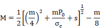
Compressive strength is calculated with the following expression:

 

 

Figure 17-A.8‑4 Tangent Line to the Hoek & Brown Failure Curve

The instantaneous friction angle will be:

The cohesion is calculated by the following expression:

 

17-A.8.3.3                        Segmentation of Material Failure Curve

The curve is divided into a series of segments defined by two stresses: S1 and S3, on the s₃ axis. The stress used to calculate the friction angle and the cohesion will be equivalent the segment defined by the average point (S1 + S3) /2.

Two critical points exist within the curve.  The first is the intersection point with the s₃ axis, which is equivalent to the tensile strength of the rock. Due to the difficulty of calculating this point, initially, the tensile strength will not be considered and s₀ = 0.

As a result, the ultimate tensile strength of the rock will be overestimated. The negative stresses will be considered by the tangent line at s₃ = 0 and therefore, the calculated stress in tension will be much higher than the actual value.

 

 

 

Figure 17-A.8‑5 Linearization in the Tensile Zone and Segmentation

The second point is s_3c, where the rock has a ductile behavior, according to Mogi studies.

 

The increment of the friction angle df controls the segmentation of the curve; to determine the angles defined from s_o  to s_3c, the following formula is used. This is dependent on s₃:

The higher and lower angles can be obtained by:

Once the f_o and f_3c angles have been determined, the curve is divided every d_f  degrees. However, the final values saved for these segments will be stresses. Therefore, in order to convert degrees into stresses, the following formula is applied to each angle:

Consequently, s₃ is calculated by:

For each pair of angles, two stresses s_inf and s_sup are generated from the lower and higher angles, respectively. The average stress between these two values will be used to approximate the curve; therefore this stress will be located at the midpoint of the section.

The stress s₃ is introduced into the following formula:

This formula will be used to calculate cohesion. First, the friction angle will be determined at the averaged point by:

 

Finally, the cohesion for this segment is obtained as:

 

17-A.8.4             Hoek & Brown Applicable Elements

The elements considered in the Hoek & Brown module are:

PLANE 42

PLANE 82

·         SOLID 45

SOLID 92

SOLID 95

The stress that is considered in each substep in order to change the material in 2D elements equals the average of the higher main stress in each node.

For the 3D elements the following expression will be applied . 

17-A.8.5             Verification Tests: Cylindrical Hole in an Infinite Hoek-Brown Medium

This problem verifies the stress distribution in an infinite elastic-plastic medium subjected to an in-situ compressive stress field of 30 MPa. 

The following material properties are assumed:

E = 10¹⁰ Pa

n= 0.25

Compression strength of 150·10⁶ Pa (intact rock).

The Hoek-Brown parameters are:

RMR = 30

m = 2.94

s = 0.01

The radius of the hole is 10 m and the model is spread 10 times more this length.

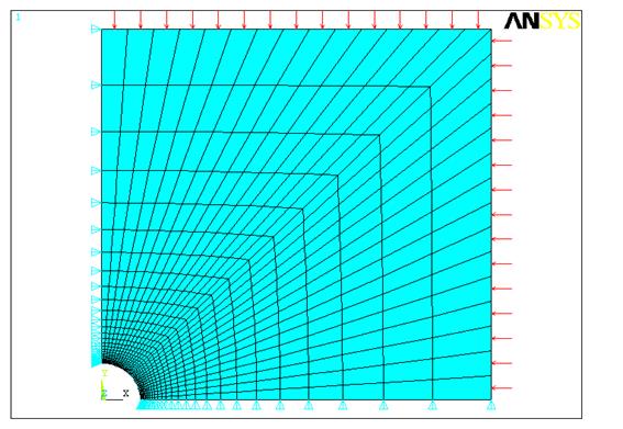
Figure 17-A.8‑6 Finite element model

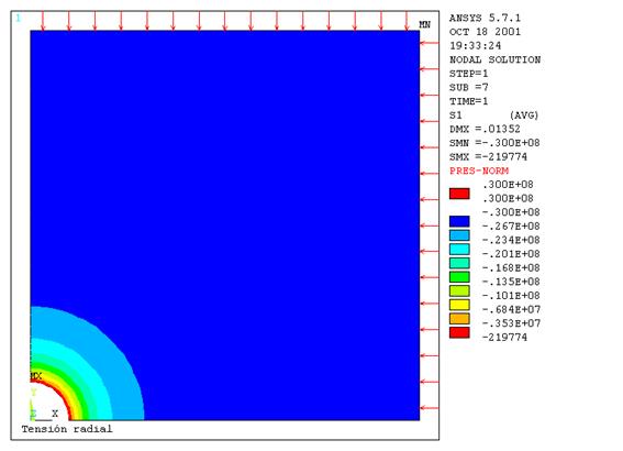
Figure 17-A.8‑7 Radial Stresses

Figure 17-A.8‑8 Tangential Stresses

 

17-A.8.6             Theoretical Solution

The theoretical solution of the tangential and radial stress distribution was studied by Hoek and Brown (Hoek and Brown Underground Excavations in Rock, London 1982).

In the elastic region:

Where

P0	Magnitude of the in-situ isotropic stress
re	Plasticity radius
	Radial stress in r = re

In the plastic region:

 

Where a is the radius of the hole and s_c is the rock compression resistance. Values s_re and r_e are defined by means of the following equation:

where

The following figure demonstrates a comparison between CivilFEM results and the theoretical results:

 

Figure 17-A.8‑9 Theoretical vs CivilFEM solution

 

17-A.9               Seepage

17-A.9.1             Introduction

The objective of this utility is to easily solve a seepage problem through a 2D or 3D porous media.

In addition, this utility performs the following actions:

• Calculation of saturation line in 2D problems.
• Export the obtained pore water pressure to the slope stability analysis. The finite element mesh can be different in both models.
• Calculation of flows through boundaries.

 

17-A.9.2             Behavior Hypothesis

It is assumed that the seepage phenomenon is governed by the following behavior hypotheses:

• Steady flow condition.
• Confined flow.
• Darcy’s law verification, with a possible anisotropy of the permeability coefficient (k is different in X, Y and Z directions).
• Permanent regime of the phenomenon (the variables that are involved are not time dependent)

 

17-A.9.3             Equation that Rules the Phenomenon

Two fields are physically defined: a scalar field of H (piezometric or hydraulic head) and a vectorial field of v (seepage velocity). An orthonormal reference S {0, xyz}, is assumed and therefore, the X axis is horizontal (permeability coefficients corresponding to k_H) and the Y axis is vertical (permeability coefficient corresponding to k_v ). With the hypotheses explained above, the following conditions are deduced:

Combining these two equations, we obtain the Laplace equation for a steady flow condition for an anisotropic soil:

 

17-A.9.4             Boundary Conditions

It is necessary to establish the boundary conditions of the following types:

Impermeable Surface

It is assumed as a flow line, therefore the seepage throughout it is null:

(Neumann type condition)

Where  is the normal to the surface.

 

Boundary with a Constant Head (Constant Head Water Load)

This part of the boundary is in contact with water and is considered as the seepage origin: 

H = H₀ (Dirichlet type condition)

Where H₀ is the total hydraulic head.

 

Seepage Surface

For the seepage surface, the pressure is atmospheric pressure:

H = piezometric height

The piezometric height axis for 2D problems is the Y axis of the global reference and the Z axis for 3D problems.

 

17-A.9.5             Calculation Results

According to the explaination in the previous sections, the equation that governs the phenomenon as well as the boundary conditions are set out in terms of the hydraulic potential h and therefore, this value is the first that provides the calculation at each node.

However, this is not the only magnitude that is of interest. The pore water pressure value as well as two more magnitudes of vectorial nature can be obtained as follows:

·         Pore water pressure

                  

·         Field gradient

·         VelocityHydraulic flow

17-A.9.6             Calculation of the Flow through a Surface

In a three-dimensional problem, the flow through a surface s is obtained by the following integration:

where  is the vector normal to the surface.

If it is a 2D problem, the unitary flow is obtained by means of a curvilinear integral:

If the arc L is a segment parallel to the axes, this integral turns into:

-          Horizontal segment [x₀, x₁]

-          Vertical segment [y₀, y₁]

 

17-A.9.7             Saturation Line (Two-Dimensional Problems)

The problem consists of obtaining the saturation line. To solve the problem, a set of areas associated with values of the “RuSi” parameter must be defined:

RuSi = 0	No seepage (uncoursed stones or precast blocks).
RuSi = 1	Seepage exists.

The RuSi parameter is obtained from the CivilFEM geotechnical database (material property). Additionally, a set of lines (polygonal lines) that identify the saturation line should be defined as an initial approximation (the program will determine the final saturation line by using the initial line as the starting point of an optimization process).

The saturation line contains two end points that comply with the following two conditions:

·         Fixed: the case for point A

·         Sliding along a seepage surface: the case of the point B.

 

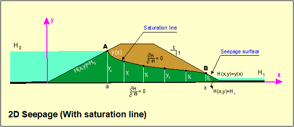
Figure 17-A.9‑1 Seepage with Saturation Line

 

17-A.9.7.1                        Operation Requirements

Geometry

A material must be assigned to each area with a defined value for the parameter “RuSi” (see ~CFMP command).

The initial saturation line will be defined as a set of lines. The intermediate points of these lines will be the control points for the saturation line calculation. CivilFEM will iterate the location of these points until the best approximation of the seepage model is achieved.

The user must set the seepage conditions of the model through the beginning and ending points (fixed or sliding) of the saturation line.

Boundary Conditions

Boundary conditions should be defined within each of the lines that create the area pertaining to the seepage phenomenon. The types of boundary conditions include:

• Constant Head condition (submerged). See ~DLHEAD command.
• Seep condition (free surface). See ~DLSEEP command.
• Null flux (impermeable surface). ANSYS default condition.

 

17-A.9.8             Export Results

A file named filename.PRESS is created to export results. These results can be used by the slope stability calculation or by the effective stresses representation. This file contains results for each node of the model.

The file structure is the following:

BLOCK 1

Version

Number of nodes

Number of elements

BLOCK 2

For each nodel of the model:

X, Y and Z coordinate; Pore pressure

BLOCK 3

I, J, K and L nodes of each element.

BLOCK 4

Adjacent elements to each element

Modifying this file could cause unpredictable results and therefore is not recommended.

 

17-A.9.9             CivilFEM Seepage Elements

The objective of this utility is to allow CivilFEM to perform the seepage analyses using CivilFEM specific finite elements (seepage elements PLANE42-SEEP and SOLID45-SEEP) without applying the thermal analogy using ANSYS thermal elements.

CivilFEM specific finite elements are similar to the ANSYS structural elements PLANE42 and SOLID45; therefore, the user may utilize all of the available resources in ANSYS for pre and postprocessing.

The corresponding CivilFEM and ANSYS elements are illustrated in the following table:

 

 

17-A.9.9.1                        Capabilities

Type of Analysis

Problems solved can be two or three-dimensional.

Boundary Conditions

Due to the objective described above, CivilFEM seepage elements can solve the Laplace equation; the resultant data is submitted to the boundary conditions that are used in the seepage problems:

-          Impermeable Boundary

(Neumann type condition)

-          Boundary with a constant head:

Commands: ~DLHEAD and ~DAHEAD.

-          Boundary with atmospheric pressure or seepage surface

H = height (Dirichlet type condition).

Commands ~DLSEEP and ~DASEEP

 

17-A.9.9.2                        Results

Results provided by CivilFEM:

·         Hydraulic head H at each node.

·         Pore water pressure u, at each point (~ISOBAR command).

This magnitude is obtained as follows: u = H – height_coordenate

·         Head gradient (¶H/¶s) at the element nodes: Components in the x, y, z directions.

·         Velocity vector at the element nodes: Components in x, y, z directions.

·         Flux or flow through each of the element faces.

 

17-A.9.9.3                        Model

The model can be constructed with ANSYS structural capabilities using the following elements:  

During the solution phase, CivilFEM will substitute these elements with CivilFEM elements with the corresponding degrees of freedom.

Thus, the user will be able to utilize all of the meshing capabilities of ANSYS Structural.

 

Element types:

 

Solution:

The CivilFEM ~LPSOLVE command must be used instead of the SOLVE command.

 

Postprocess

When CivilFEM seepage elements are used, the results file generated is jobname.SEEP.  Therefore, to access these results, the user must execute the command FILE, jobname, SEEP followed by the command SET, 1 to access the solved load step. The CivilFEM seepage elements only withstand one load step, always stored as the first load step.

The plots and listings can be obtained by standard ANSYS commands using the CivilFEM degree of freedom HEAD. For example PLNSOL, HEAD, plots the head contours.

In addition, the ~LPRNSOL command lists the nodal results. The seepage commands ~PLSEEP and ~ISOBAR plots the seepage and the pore water pressure results respectively; these commands function as usual with these new elements.

Element results are obtained from the integration points and then interpolated in the nodes. See section 13.6 “Nodal and Centroidal Data Evaluation” in the ANSYS’s Theory Reference manual.

 

17-A.9.9.4                        Element Descriptions

 

·         Plane42-SEEP

This element is a variation of the structural element PLANE42 with the capability of solving seepage problems.

PLANE42-SEEP can be used as a plane element with two-dimensional seepage capabilities. The element has four nodes with a single degree of freedom: the hydraulic head at each node.

The element can be utilized for a 2D steady-state seepage analysis.

Figure 17-A.9‑2 PLANE42-SEEP Element

Input Data

The element is defined by four nodes and the material properties KXX, KYY and KZZ. Orthotropic material directions correspond to the global coordinate directions.

Input Summary

Element Name

PLANE42-SEEP

Nodes

I, J, K, L

Degrees of Freedom

HEAD

Material Properties

KXX, KYY, KZZ.

Output Data

The solution data for the element is outputted in two forms:

·         Nodal heads included in the overall nodal solution

·         Element output as shown in Element Output Definitions

The nodal solution can be obtained using the HEAD label of the PLANE42-SEEP element.

Result arguments can be obtained by the component name method [ETABLE, ESOL]. The name of the results file is Jobname.SEEP; therefore, the user must issue the command FILE,filename,SEEP to read the results.

The PLANE 42-SEEP equivalence column in the table below lists the names of PLANE42 used to obtain the results.

The following arguments are available in the results file:

Table 17-A.9‑1 PLANE42-SEEP Element Output Definitions

 

The following table shows the sequence numbers for obtaining results using the ETABLE and ESOL commands:

Table 17-A.9‑2 PLANE42-SEEP Item and Sequence Numbers for the ETABLE and ESOL Commands

 

Name

Output quantity as defined in the Element Output Definitions

Item

Predetermined Item label for ETABLE command

FCn

Sequence number for solution items for element face n

Assumptions and Restrictions

The area of the element may not be zero or negative and the element must be located on the X-Y plane.

Product Restrictions

This element can only be used with the CivilFEM Geotechnical Module.

 

• SOLID45-SEEP

This element is a variation of the SOLID45 structural element, capable of solving seepage problems.

SOLID45-SEEP can be used as a solid element with three-dimensional seepage capabilities. The element has eight nodes with a single degree of freedom: hydraulic head at each node.

This element can be utilized for a 3D steady-state seepage analysis.

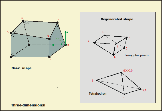
Figure 17-A.9‑3 SOLID45-SEEP Seepage Element

Input data

The element is defined by eight nodes and by the material properties KXX, KYY and KZZ. Orthotropic material directions correspond to the global coordinate directions.

 

Input Summary

Element Name

SOLID45-SEEP

Nodes

I, J, K, L, M, N, O, P

Degrees of Freedom

HEAD

Material Properties

KXX, KYY, KZZ

 

Output Data

The solution data for the element is outputted in two forms:

·         Nodal heads included in the overall nodal solution

·         Element output as shown in Element Output Definitions

The nodal solution can be obtained using the UX label of the SOLID45 element.

Result arguments can be obtained by the component name method [ETABLE, ESOL]. The name of the results file is Jobname.SEEP; therefore, the user must issue the command FILE,filename,SEEP to read the results.

In the table below, the SOLID45-SEEP equivalence column lists the names of SOLID45 used to obtain the results.

The following arguments are available in the results file:

Table 17-A.9‑3 SOLID45-SEEP Element Output Definitions

 

The following table shows the sequence numbers for obtaining results using the ETABLE and ESOL commands:

Table 17-A.9‑4 SOLID45-SEEP Item and Sequence Numbers for the ETABLE and ESOL Commands

Name	Item	FC1	FC2	FC3	FC4	FC5	FC6
PRES	SMISC	1	2	3	4	5	6

 

Name

Output quantity as defined in the Element Output Definitions

Item

Predetermined Item label for ETABLE command

FCn

Sequence number for solution items for element face n

Assumptions and Restrictions

The volume of the element may not be zero. The geometry of the elements will be numbered as SOLID45 elements. Also, the element may not be twisted such that it forms two separate volumes. This occurs most frequently when the elements are not numbered properly.

All elements must have eight nodes. A prism-shaped element may be formed by defining duplicate K and L and duplicate O and P node numbers (see triangle, prism and tetrahedral elements). A tetrahedron shape is also available. The extra shapes are automatically deleted for tetrahedron elements.

Product Restrictions

This element can only be used within the Geotechnical Module.

 

 

17-A.10         Earth Pressures

17-A.10.1         Introduction

CivilFEM provides the user with a series of commands that allows to apply directly the pressures and forces corresponding to the active, passive and at rest earth pressure and the soil weight of the defined terrain, on the selected model elements.

17-A.10.2         Element Types

CivilFEM can apply earth pressures to the following elements:

2D Beam Elements

            BEAM3, BEAM23, BEAM54

3D Beam Elements

            BEAM4, BEAM24, BEAM44, BEAM188, BEAM189

Shell Elements

            SHELL43, SHELL63, SHELL93, SHELL181

2D Solid Elements

            PLANE2, PLANE42, PLANE82, PLANE145, PLANE146

3D Solid Elements

            SOLID45, SOLID46, SOLID64, SOLID65, SOLID73, SOLID95, SOLID147

Surface Elements

            SURF153, SURF154

 

17-A.10.3         Terrain Definition

The definition of a terrain is necessary for calculating earth pressures (~TERDEF command).

The terrain can have different layers.

 

17-A.10.4         Earth Pressure

Calculation Hypotheses

The active or passive earth pressure calculation is performed using either Coulomb’s theory (if specified in the layer definition of the terrain), or the material data base pressure coefficients (Rankine theory by default). The at rest earth pressure uses the material data base pressure coefficients. The earth pressure is produced by the sliding of a soil wedge, bounded by the back face of the retaining wall or similar structural element and a plane that goes through the foot of the element. This theory makes the following assumptions:

·         The ground does not have cohesion.

·         The earth surface is flat. The angle between the surface and the horizontal is called b,  and q is the surcharge pressure per unit area, measured along the slope.

·         Neither the pressure reduction due to other walls that limit the maximum pressure wedge nor the possible silo effect will be considered.

·         The pressure on isolated elements will be calculated with their real width; consequently, for elements with a small width, the corresponding pressure will not be increased by increasing its width.

Calculation Process

Earth pressure calculation and application on the selected elements will follow these steps:

1. Obtaining the angle a for each one of the selected elements. The angle a is between the face of the element on which the pressure is applied and the horizontal line of the earth. This angle is measured on the opposite side that the pressure is applied.

In beam elements, this angle is calculated in the element axis direction; therefore, it is calculated with the direction given by the end nodes (considering the 3^rd node or the orientation angle TETHA in 3D beam elements). Hence, for beams with variable cross-sections, the a angle will slightly differ from reality.

In shell elements, the angle a is calculated from the plane formed by the first three nodes of the element. As for beam elements, for shells with variable thickness, this angle will slightly differ from the actual value.

For 2D and 3D solid elements, the angle a is obtained from the first three nodes of the face on which the pressure is applied; in this case, the angle will always be the actual value.

In order for a to be within the valid range for earth pressure coefficient equations and for the physical problem to make sense, a must satisfy the following:

2.    Calculation of the earth pressure coefficients. Once the angle a has been calculated from the defined values of the soil, the earth pressure coefficients will be obtained from the data base or from Coulomb’s theory, according to the theory explained in chapter 17-A.4.5 Earth Pressure over the wall.

In the following sections, the earth pressure coefficient will be referred to as K, independent of the type of pressure is applied (active, passive, etc.):

3.    Calculation of normal and tangential pressures.

 

For dry earth without a surface load, pressures located on a point at a depth z beneath the surface are obtained with the following expression:

This pressure per unit depth will form an angle d (Soil-wall friction angle) with the face of the element.

As a result, the total force applied to a differential element will be:

Consequently, the pressure on this differential element along the element direction will be:

Figure 17-A.10‑1 Earth Pressure Application

By projecting this pressure on the element, the following is obtained:

 

If there is a uniformly distributed load on the soil of value q per unit length of sloped soil, the pressure located on a point at a depth z beneath the ground surface is:

Hence, normal and tangential pressures on the element are calculated by:

For flooded earth, the pressure beneath the water table is calculated with the specific weight:

If f is the depth of the water table, the pressure at a depth z (higher than the water table depth) is obtained by:

Consequently, the normal and tangential pressures on the element are:

4.    Application of normal and tangential pressures on elements.

Beam and Surf153 Elements

For these elements, normal and tangential pressures are directly applied onto each element. For beam elements, the thickness of the element will be obtained from the Cross Sections assigned to the Beam Properties. If the element is a tapered beam, the mean value of the thickness for each cross section will be used.

Shell, Solid and Surf154 Elements

For these elements, the normal pressure is applied directly, and the tangential pressure is applied through forces on the nodes in the tangential direction. The forces on the nodes are calculated multiplying the tangential pressure by the area associated with each node, according to the selected elements. When the node coincides with angle a variation, a force is applied that is the average of the forces, in magnitude as well as in direction, that correspond to the node for each value of the angle a  .

17-A.10.5         Pressure due to Soil Weight

Calculation Hypotheses

The pressure due to the soil weight is calculating from weight of the soils over the element and the overload on the ground surface. Consequently, the following statements are assumed:

·         A normal and a tangential pressure are applied to elements with a vertical resultant.  The pressure due to the water is only applied normal to the element.

·         The ground surface is flat, forming an angle b with the horizontal and with an overload q per unit area, measured along the slope of the soil.

·         The pressure reduction due to the possible silo effect with other elements is not considered.

·         The pressure on insolated elements is calculated considering the element real width.

Calculation Process

The calculation and application of pressure due to the soil weight on the selected elements, follows these steps:

1.    Obtain the angle a for each selected element, as demonstrated for the earth pressure calculation.

2.    Calculate the normal and tangential pressure.

For dry earth without a surface load, the pressure values due to the soil weight on a point at a depth z is the following:

Projecting this pressure on the element obtains:

Figure 17-A.10‑2 Earth Pressure Application

If there is a uniformly distributed load on the soil with value q per unit length of sloped soil, the pressure value on a point at a depth z beneath the ground surface is:

 

For flooded grounds, the pressure beneath the water table is calculated with the specific weight:

If f is the depth of the water table, the pressures at a depth z (higher than the water table depth) will be obtained by:

3.    Apply the normal and tangential pressures on elements. Pressures are applied as explained in the earth pressures calculation.

17-A.11         Terrain Initial Stress

17-A.11.1         Description of the Stress State

Initial stress without strain is introduced into CivilFEM via the ~TIS command.

In geotechnics, it is common to work with an initial stress state with a horizontal component is proportional to its vertical component.

Figure 17-A.11‑1 Stresses in a Differential Element

The k_o parameter is known as the at rest earth pressure coefficient as well as the horizontal earth pressure coefficient. This value depends upon the material and its degree of consolidation.

 

17-A.11.2         Value of the At Rest Earth Pressure (K₀)

17-A.11.2.1                     Elastic Theory

From the equation:

In a Boussinesq semispace (horizontal soil), loaded with a uniform load (for example its self weight), the following relationship occurs:

and therefore:

Hence:

Consequently:

In the table and graphs shown below, the range of the k_o coefficient with the Poisson modulus is represented; these figures conclude that the elastic theory never exceeds values greater than 1 for k_o.

 

 

 

17-A.11.2.2                     Friction Angle Dependency

For normally consolidated soils the k_o coefficient may be approximately obtained from the following equation suggested by Jaky:

Where the parameter j is the material friction angle, expressed in effective stresses.

 

17-A.11.2.3                     Experimental Values

The first studies conducted to measure the value of the at rest earth pressure (k₀ coefficient) are attributed to Karl Terzaghi, who during the years 1920 and 1925 published the following values.

 

 

It appears as if the proposed values for sands are sometimes too small and those for clays are too big. Today, awaiting new studies regarding this matter, the following values are considered acceptable:

 

 

In addition, the required values j and u to obtain the at rest earth pressure are represented in the table above.

Due to their nature, both equations cause k₀ coefficient values to be lower than the one. However, in high-consolidated clays the k₀ coefficient has been measured by using indirect methods to produce values between 2 and 4 (Skempton 1961, Bishop 1965); this result has been repeated in other material types.

These values cannot be reproduced with the equations seen in the previous sections.

 

17-A.11.3         Initial Stresses

From a given topography, the initial stresses will be calculated by:

With h as the depth of the point considered, g as the specific weight of the material and k₀ as the at rest earth pressure coefficient.

In the case of a layered soil of n materials located over the considered point, the previous expressions would be:

 

17-A.11.4         Obtaining an Initial Stress File

The ~TIS command generates an ASCII file with the values of initial stresses at the center of the elements. These values are calculated in function of the active (cartesian) coordinate system.

The initial stresses are introduced into the model by reading the initial stresses file. This file must be compatible with the type of element, which is controlled by the argument KTIS of the command ~TIS

Since INISTATE command is not longer supported, it is suggested to define initial stresses on the element types 182, 183, 185, 186 and 187.

It is recommended to solve a first load step with the initial stressed and the self-weight. Thus, the initial stresses introduced will be adjusted to create a balanced stress with the gravity. A slight variation may occur between the introduced stresses ant the stresses from equilibrium.