8.1                       Structure’s Cost and Weight

8.1.1                      Cost

The cost per unit volume of the CivilFEM materials defined in a structure is used for the computation of the cost of each element in that structure.

This value is only an approximation of the real cost of the structure since it does not account for precise details or final, exact geometry of complex structures. Nevertheless, it is especially useful in optimization analyses in which the broad, global cost of the structure must be minimized.  

The cost of each element is computed as follows:

• Volumetric elements (SOLID): The volume of the element is multiplied by the cost per unit volume corresponding to its material.
• Linear elements (BEAM, LINK): The cost of the cross section is calculated from the cost values of its different materials and the discretization into tessella and plates; this cost accounts for the gross section formulation, not the effective section. The total cost of the element will be the arithmetic mean of the costs of each cross section (one for each end), multiplied by its length.
• Shell elements: For linear elements, the cost of each end (shell vertex) is added with cost of the reinforcement amount for each of the concrete vertices; the mean value between these costs will be the total cost of the element.

Shear and torsional reinforcement (beams and shells) are not considered in the cost calculation.

The cost can be obtained accounting for each material (~COSTLST command) or can be used as a variable in the analysis (~COST command).

The elements meshed using a generic ANSYS material will not be considered for the cost calculation.

8.1.2                      Weight

It is sometimes necessary to determine the weight of the structure, which can be obtained in two ways:

• From the geometry of the structure and the densities of the materials used.
• From adding the reactions on the supports, once the model is solved.

The second method can lead to errors when coupling equations are used between nodes, supports are rotated, etc.

The first method can be directly applied using the ~WEIGHT command. Its calculation procedure is the same as the cost computation procedure, but it uses the specific weight of each material instead of the cost per unit volume.

Elements meshed using a generic ANSYS material will not be considered for the weight calculation according to the first method.

 

 

8.2                       Influence Lines

8.2.1                      Range and Restrictions

It is possible to obtain influence lines in 2D and 3D beam structures in which the model is meshed using BEAM188 and BEAM189 elements.

For a given 3D structure, up to 36 different influence lines can be obtained; this value is the result of combining any of the six target forces and moments (FX, FY, FZ, MX, MY, MZ) with six possible actions (FX, FY, FZ, MX, MY, MZ). For 2D structures the number of possible influence lines is nine (FX, FY, MZ) vs (FZ, MY, MZ).

The definition of the orientation of the elements must be done using the third node K.

It is important to point out that the forces and moments, both targeted and applied, always refer to the nodal coordinate systems.

To obtain the influence line, CivilFEM uses the reciprocal theorem of the Müller-Breslau Principle; therefore, it is necessary to temporarily alter the structure.

Because of its nature, the influence line cannot be calculated for nodes other than those connected to two, and only two, beams.

8.2.2                      Opening and Closing Influence Lines

As stated before, the structure must be altered temporarily in order to obtain the influence line. Therefore, degrees of freedom may be released, beams may be unconnected, etc.

CivilFEM will alter the structure when the influence line is created (the opening of the influence line, ~ILOPEN command). The program will restore the model to its initial geometry and conditions either immediately after the line has been calculated or sometime after (~ILCLOSE command) in order to postprocess the results of the influence line.

8.2.3                      Assemblies

When an influence line has been created, the following assemblies are created:

• CFInfLine%ILID%POSITIVE
• CFInfLine%ILID%NEGATIVE

Where %LID% is the number of the created influence line.

These assemblies contain nodes and elements on which a load (force, moment or pressure) that acts on them has a positive or negative effect on the target force or moment.

It is important to note that pressures on beam elements will act perpendicular to these elements, in a direction that depends on the element axis (as well as the locations of the I, J, K nodes); therefore, it is advisable to pay attention its definition, in relation to the nodal coordinate system.

8.2.4                      Examples

8.2.4.1                  Description

In order to help the user become more comfortable with the use of influence lines, five examples have been prepared. These examples are followed by sketches of the structure and log files:

 

-          Example 1

A continuous horizontal beam contains five spans, and influence lines at a point in the middle of a span are obtained for the bending moment and the shear force.

There is an applied vertical force, FY.

This example as well as the following one are very simple and serve as introductions to this utility.

 

-          Example 2

With the same structure as the previous example, the influence lines at a point located at a support are obtained for the bending moment and shear force. The applied vertical force FY is maintained.

 

-          Example 3

This structure consists of a plane, fixed-end, circular arch. Influence lines at a non-centered midpoint are obtained for the bending moment and the shear and axial forces

The applied force is perpendicular to the arch.

The purpose of this example is to become familiar with nodal coordinate systems.

 

-          Example 4

On a plane frame, a surface load has multiple possible locations of application as shown in the corresponding sketch.

The objective is to obtain the surface load location that will create the maximum negative bending moment at the specified point.

Nodal coordinate systems are used in this example as well; however, these systems are coordinated with the element coordinate system.

Once the influence line has been obtained, the assembly which contains the elements that generate the negative bending moment on the node will be loaded, and the structure will be solved.

In this example tolerances are also used (NEGTOL). It is recommended to practice this example with different values for this field.

 

 

-          Example 5

In this last example, the loads on a three dimensional structure, located on a plane, act perpendicular to the plane in the –Z direction.

The objective of this example is to obtain the influence line of the torsional moment.

 

8.2.4.2                  Example 1. Five Span Continuous Beam

 

Sketches

 

LOG

 

 

8.2.4.3                  Example 2. Five Span Continuous Beam

 

Sketches

LOG

 

 

8.2.4.4                  Example 3. Fixed-end Circular Arch

 

Sketches

LOG

 

 

 

8.2.4.5                  Example 4. Three Leg Frame

 

Sketches

 

LOG

 

 

 

8.2.4.6                  Example 5. 3D Plane Structure

 

Sketches

LOG

 

8.3                       Solid to Shell

8.3.1                      Introduction

In finite element analyses it is common to model reinforced concrete or prestressed concrete structures using 3D solid elements to determine the stresses at the nodes of elements.

 Nevertheless, codes and standards in the majority of the cases and countries utilize forces and moments for the calculations, either for shell or beam elements.

CivilFEM includes a utility (SOLID SECTION) that integrates stresses obtained from a model in order to convert them into beam forces and moments; these stresses are assumed to be prismatic.

For 3D solid element structures that are assumed to be laminar, this utility will obtain the forces and moments necessary to apply codes or standards which are based on these values.

 

8.3.2                      Initial Data

It is necessary to define the following types of data:

• Structure (complete or partial), already defined by 3D solid elements.
• Necessary information for the definition of the shell elements.

The definition of the structure to be analyzed is the first required data. It must be defined by two components:

• Nodes of a surface (external or internal) of the structure.
• All the elements that form the structure.

The following figure illustrates these requirements.

 

Apart from this, to define the reinforced concrete shells, it is necessary to define the cover that will be used and the material for the reinforcement.

From this information, CivilFEM creates a new component with dummy SHELL181 elements, at the mid-surface of the 3D structure that will be the base to obtain the needed results. These elements will also be used for the results.

The dummy shell elements have materials and shell properties assigned, which CivilFEM creates from the material of the solid structure and the thicknesses. The created material will add no mass to the structure so it does not interfere in inertial or transient analyses.

These new shell elements are defined on nodes created independently from the existing model. These nodes have all their degrees of freedom constrained.

Moreover, this utility generates the following components:

CF_SD2SH_NODES_#: generated nodes component of dummy shells group number #.

CF_SD2SH_ELEMENTS _#: generated elements component of dummy shells group number #.

 

 

8.3.3                      Calculation of the Shells’ Thicknesses

From the center of gravity of the outer element surfaces, CivilFEM casts rays, perpendicular to this surface, which intersect the different elements of the structure (hexahedra, tetrahedra or pyramids) at two of their faces (upon entry and exit) shown as points 1 and 2 in the following figure.

 

 

If the ray is not perpendicular to the outer surface, CivilFEM will correct the ray’s direction so that its vector is the mean value of the perpendicular vectors to the entry and exit surfaces. But if the ray exits through a lateral surface, instead of the opposite face, the direction of the ray will be parallel to this lateral face.

Instead of using this perpendicular direction to define the integration planes, a local coordinate system can be used. In this case, the ray will follow the direction of the Z axis of the local coordinate system and will also orientate the element axis of the dummy shells to be parallel to this coordinate system. If the direction of the Z axis is 5º away from the mean value of the entry and exit vectors, CivilFEM will show it in the error file CF_SD2SH.ERR and a warning will be issued with the number of the elements on which this warning applies.

In this process, the thickness d of the structure is obtained for each analyzed section. This value can be rounded according to a certain tolerance given in each case or to a certain value. If a constant thickness is set by the optional argument TH of the command ~SD2SH and the obtained thickness is different, CivilFEM will display this in the error file CF_SD2SH.ERR and a warning will be issued with the number of the elements for which this warning applies.

If any dummy shell element cannot be generated, CivilFEM will record this in the error file CF_SD2SH.ERR, indicating the outer solid element number of the outer surface used to generate the shell element.

8.3.4                      Calculation of the Stress Tensor

During the procedure to obtain the thicknesses of the shell elements, each casted ray defines calculation points in space (the entry and exit points of each solid element). The calculation of the stress tensor at each of these points is accomplished by interpolation from the nodes of the faces.

A group of stress tensors is obtained:

Where n is the number of elements faces the ray went through.

In SOLID65 elements, stresses are only read from the nodes and tension at rebars is not taken into account.

8.3.5                      Calculation of Forces and Moments

 

8.3.5.1                  Axial Forces

 

The axial force in the X direction can be calculated as:

 , t = thickness direction

Where the values of d_i are the distances from the calculation points to the center of the dummy shell element.

In the same way, the Y direction is calculated as:

 

8.3.5.2                  Bending Moments

 

The bending moment is the static moment of the stress function from an axis at the center of the section:

Where x is the distance from each point to the center. To calculate the moments, the following equation is used:

 

8.3.5.3                  Shear Forces

 

Defined by the integration of the t_xy and t_yz stresses:

 

8.3.5.4                  Sliding Shear Force

 

Obtained by using the following expression:

 

8.3.5.5                   Torsional Moment

 

Obtained from the following expression:

 

8.3.6                      Results of the Dummy Shell Elements

The dummy shell elements can be postprocessed in the same way as any other element of the structure. However, their nodes have no stress or movement results.

Since the results of these elements are forces and moments, it is possible to perform code checks on them. Data from the code checks will be stored in the results file to be postprocessed as with any other shell element.

To apply reinforcement to the structure, the axes of the shell elements must be oriented in the same direction as the reinforcement bars. If the dummy shell elements have not been oriented by the command argument, this orientation must be defined after they have been created.

 

8.3.7                      Remesh

 

In order to increase the accuracy of the analysis, it is possible to remesh the exterior elements of the dummy shell group. The remesh level varies between 1 and 3, where 3 is the finest remesh. For the finest level, the exterior elements are divided into 26 or 29 new elements, depending on if a triangular or a quadrangular shape is used for the division. The remesh increases the number of calculation points while decreasing the distances from these points to the boundary. Consequently, the boundary behavior is captured with a higher accuracy.

 

8.4                       Concrete Relax Procedure

8.4.1                      Introduction

This post processing method has been developed to take into account the cracked mechanical properties and redistribution of stresses of concrete shells. This procedure can be used to reduce forces and moments created by strain-dependent loads. For example:

-          Thermal load

A temperature increment ΔT in a beam will generate the strain ε= α. ΔT

In a constrained model, this strain will generate an axial force:

N= A. E. ε

This axial force is proportional to the section stiffness K== A. E

When gross inertia is computed then N_GROSS= A_GROSS. E. ε

When the cracked area is computed, N_CRACKED= A_crack. E. ε

Therefore N_CRACKED= N_GROSS (A_crack /A_GROSS)

-          Footing settlement

In the same way, when analysing the bending moment that is produced on a column due to a rotation angle φ of the footing, then:

Bending moment will be proportional to the column stiffness M= E.I.φ

When gross inertia is computed, then M_GROSS= E.I_GROSS. φ

When the cracked area is computed, then M_CRACKED= E.I_crack. φ

Therefore M_CRACKED= M_GROSS (I_crack /I_GROSS)

 

8.4.2                      Initial Data

User has to define initial data which are the mechanical loads that are acting with strain-dependent loads, so different load steps must be defined for each kind of load (mechanical loads and strain-dependent loads).

Command ~CFFILE2, 5, Name, LS, SS must be used to indicate the software the mechanical loads used to reduce strain-dependent loads, where Name is the name of the result file and LS and SS, the load step and substep.

8.4.3                      Calculation of crack ratio

In the first interaction, the cracked properties (neutral axis, inertia I₁ and area S₁) are obtained on every section for the mechanical loads. If cracks occur, resulting area and inertia are smaller than the initial gross cross section inertia and area (I₀ and S₀) which where used in solution level.

If thermal loads cause cracking in the same face than the mechanical loads, that is, bending moments have the same sign, new strain-dependent forces are calculated  obtained by multiplying the bending moment by the I₁/ I₀ ratio and the axial force by the S₁/ S₀ ratio. That is, reduced bending moment and axial force are calculated with the following formula:

                        M₁= M₀ (I₁/I₀)

                        N₁= N₀ (S₁/S₀)

If bending moments have different sign, the thermal loads could close the crack, therefore, it is conservative to consider the gross section:

                        M₁= M₀

                        N₁= N₀

After that, with an iterative procedure, inertia and area are re-calculated for the new combinations considering the reduced axial force and bending moment M₁ and N₁

The model will converge when

(I_i+1/I_i)< (1+tolerance) and (S_i+1/S_i)< (1+tolerance).

 

8.4.4                      How To Use Results

Results of forces and moments reduced are stored in a new data set in CivilFEM results file. To launch the process and store these values, user must follow the next steps:

1-    Set initial data (mechanical data set) with ~CFFILE2 command

2-    Duplicate ANSYS data set of the results for strain-dependent loads with command RAPPND and point to this result with SET ANSYS command.

3-    Launch concrete relax procedure with command ~MOD_SF,,CONRELAX

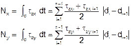
Results are stored in a new data set in CivilFEM. Bending and axial crack ratios in both directions (ratio_M_X, ratio_N_X, ratio_M_Y, ratio_N_Y) are used to obtain the new forces and moments:

 

Tx	Tx* ratio_N_X
Ty	Ty* ratio_N_Y
Txy	Txy* MIN(ratio_N_X, ratio_N_Y)
Mx	Mx* ratio_M_X
My	My* ratio_M_Y
Mxy	Mxy* MIN(ratio_M_X, ratio_M_Y)
Nx	Nx* ratio_M_X
Ny	Ny* ratio_M_Y